Multi-fidelity Monte Carlo

This tutorial builds on from Multi-level Monte Carlo and Two model Approximate Control Variate Monte Carlo and introduces an approximate control variate estimator called Multi-fidelity Monte Carlo (MFMC) [PWGSIAM2016].

To derive the MFMC estimator first recall the two model ACV estimator

\[Q_{0}^\mathrm{MFMC}(\rvset_\text{ACV})=Q_{0}(\rvset_{0}) + \eta\left(Q_1(\rvset_{1}^*)-Q_{1}(\rvset_{1})\right)\]

The MFMC estimator can be derived with the following recursive argument. Partition the samples assigned to each model such that \(\rvset_\alpha=\rvset_{\alpha}^*\cup\rvset_{\alpha}\) and \(\rvset_{\alpha}^*\cap\rvset_{\alpha}=\emptyset\). That is the samples at the next lowest fidelity model are the samples used at all previous levels plus an additional independent set, i.e. \(\rvset_{\alpha}^*=\rvset_{\alpha-1}\).

Starting from two models we introduce the next low fidelity model in a way that reduces the variance of the estimate \(Q_{\alpha}(\rvset_\alpha)\), i.e.

\[\begin{split}Q_{0}^\text{MFMC}(\rvset_\text{ACV})&=Q_{0}(\rvset_{0}) + \eta_1\left(Q_{1}(\rvset_{1}^*)-\left(Q_{1}(\rvset_{1})+\eta_2\left(Q_{2}(\rvset_2^*)-Q_{2}(\rvset_{2})\right)\right)\right)\\ &=Q_{0}(\rvset_{0}) + \eta_1\left(Q_{1}(\rvset_{1}^*)-Q_{1}(\rvset_{1})\right)+\eta_1\eta_2\left(Q_{2}(\rvset_2^*)-Q_{2}(\rvset_{2})\right)\end{split}\]

We repeat this process for all low fidelity models to obtain

\[Q_{0}^\text{MFMC}(\rvset_\text{ACV})=Q_{0}(\rvset_{0}) + \sum_{\alpha=1}^M\eta_\alpha\left(Q_{\alpha}(\rvset_{\alpha}^*)-Q_{\alpha}(\rvset_{\alpha})\right)\]

The allocation matrix for three models is

\[\begin{split}\begin{bmatrix} 0 & 1 & 1 & 1 & 1 & 1 & 1 & 1\\ 0 & 0 & 0 & 1 & 1 & 1 & 1 & 1\\ 0 & 0 & 0 & 0 & 0 & 1 & 1 & 1\\ 0 & 0 & 0 & 0 & 0 & 0 & 0 & 1 \end{bmatrix}\end{split}\]

The optimal control variate weights and the covariance of the MFMC estimator can be computed with the general formulas presented in Approximate Control Variate Monte Carlo.

Optimal Sample Allocation

Similarly to MLMC, the optimal number of samples that minimize the variance of a single scalar mean computed using MFMC can be determined analytically (see [PWGSIAM2016]) provided the following condition is met

\[\frac{C_{\alpha-1}}{C_\alpha} > \frac{\rho^2_{0,\alpha-1}-\rho^2_{0,\alpha}}{\rho^2_{0,\alpha}-\rho^2_{0,\alpha+1}}\]

When this condition is met the optimal number of high fidelity samples is

\[N_0 = \frac{C_\mathrm{tot}}{\V{C}^T\V{r}}\]

where \(\V{C}=[C_0,\cdots,C_M]^T\) are the costs of each model and \(\V{r}=[r_0,\ldots,r_M]^T\) are the sample ratios defining the number of samples assigned to each model, i.e.

\[N_\alpha=r_\alpha N_0.\]

The number in each partition can be determined from the number of samples per model using

\[p_0 = N_0, \qquad p_\alpha=N_\alpha-N_{\alpha-1}, \;\alpha > 0.\]

Recalling that \(\rho_{j,k}\) denotes the correlation between models \(j\) and \(k\), the optimal sample ratios are

\[r_\alpha=\left(\frac{C_0(\rho^2_{0,\alpha}-\rho^2_{0,\alpha+1})}{C_\alpha(1-\rho^2_{0,1})}\right)^{\frac{1}{2}}.\]

Now lets us compare MC with MFMC using optimal sample allocations

import numpy as np
import matplotlib.pyplot as plt

from pyapprox.util.visualization import mathrm_labels
from pyapprox.benchmarks import setup_benchmark
from pyapprox.multifidelity.factory import (
    get_estimator, compare_estimator_variances, compute_variance_reductions,
    multioutput_stats)
from pyapprox.multifidelity.visualize import (
    plot_estimator_variance_reductions)

np.random.seed(1)
benchmark = setup_benchmark("polynomial_ensemble")
model = benchmark.fun
cov = benchmark.covariance
target_costs = np.array([1e1, 1e2, 1e3, 1e4], dtype=int)
costs = np.asarray([10**-ii for ii in range(cov.shape[0])])
model_labels = [r'$f_0$', r'$f_1$', r'$f_2$', r'$f_3$', r'$f_4$']

stat = multioutput_stats["mean"](benchmark.nqoi)
stat.set_pilot_quantities(cov)
estimators = [
    get_estimator("mlmc", stat, costs),
    get_estimator("mfmc", stat, costs)]
est_labels = mathrm_labels(["MLMC", "MFMC"])
optimized_estimators = compare_estimator_variances(
    target_costs, estimators)

axs = [plt.subplots(1, 1, figsize=(8, 6))[1]]

# get estimators for target cost = 100
ests_100 = [optimized_estimators[0][1], optimized_estimators[1][1]]
_ = plot_estimator_variance_reductions(
    ests_100, est_labels, axs[0])

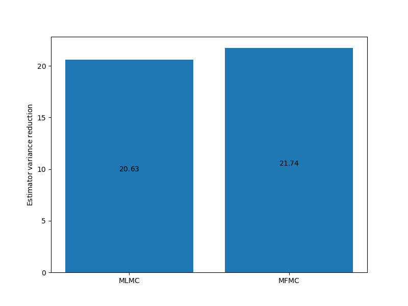
For this problem there is little difference between the MFMC and MLMC estimators but this is not always the case.

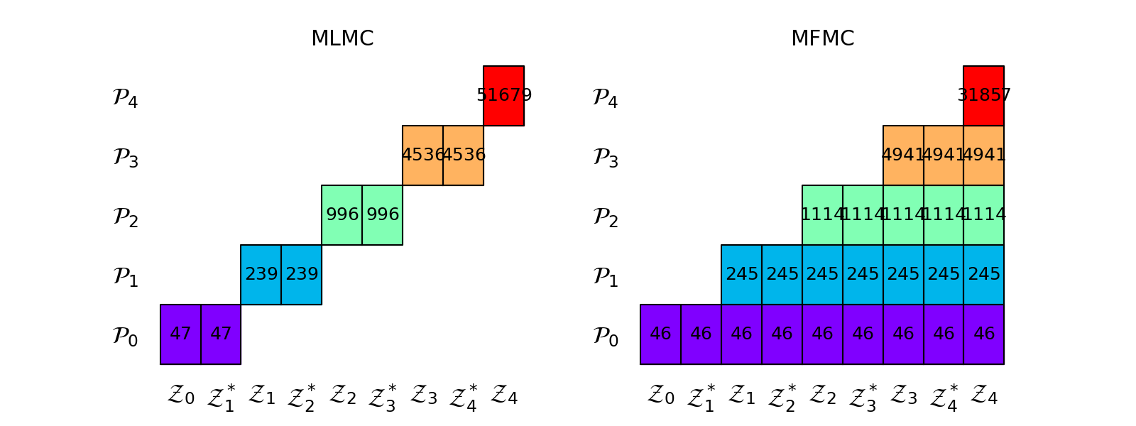
The following plots the sample allocation matrices of the MLMC and MFMC estimators

import matplotlib as mpl
params = {'xtick.labelsize': 24,
          'ytick.labelsize': 24,
          'font.size': 18}
mpl.rcParams.update(params)
axs = plt.subplots(1, 2, figsize=(2*8, 6))[1]
ests_100[0].plot_allocation(axs[0], True)
axs[0].set_title(est_labels[0])
ests_100[1].plot_allocation(axs[1], True)
_ = axs[1].set_title(est_labels[1])

Comparison To Control Variates

It is clear from the recursive derivation of MFMC above that MFMC uses model \(m\) as a contol variate to help estimate the statistic of model \(m-1\). Not all models are directly used to reduce the variance of \(Q_0\); MLMC admits has the same property. The effect of the recursive property of MFMC and MLMC can be observed with the following code.

Below we we plot the ratios \(\var{Q_0^\text{MFMC}(\rvset_\text{MFMC})}/\var{Q_0^\text{MC}(\rvset_0)}\) and \(\var{Q_0^\text{MLMC}(\rvset_\text{MLMC})}/\var{Q_0^\text{MC}(\rvset_0)}\) as we increase the number of samples assigned to the low-fidelity models, while keeping the number of high-fidelity samples fixed. We also plot \(\var{Q_0^\text{CV}(\rvset_0)}/\var{Q_0^\text{MC}(\rvset_0)}\) for control variate estimator that use increasing numbers of models with known low-fidelity statistics. These CV-based variance ratios represent the best ACV estimators could possibly do if the cost of evaluating the low-fidelity models was zero.

nhf_samples = 1
nmodels = costs.shape[0]

cv_stats, cv_ests = [], []
for ii in range(1, nmodels):
    cv_stats.append(multioutput_stats["mean"](benchmark.nqoi))
    cv_stats[ii-1].set_pilot_quantities(cov[:ii+1, :ii+1])
    cv_ests.append(get_estimator(
        "cv", cv_stats[ii-1], costs[:ii+1],
        lowfi_stats=benchmark.mean[1:ii+1]))
cv_labels = mathrm_labels(["CV-{%d}" % ii for ii in range(1, nmodels)])
target_cost = nhf_samples*sum(costs)
[est.allocate_samples(target_cost) for est in cv_ests]
cv_variance_reductions = compute_variance_reductions(cv_ests)[0]

from util import (
    plot_control_variate_variance_ratios,
    plot_estimator_variance_ratios_for_polynomial_ensemble)

ax = plt.subplots(1, 1, figsize=(8, 6))[1]
plot_control_variate_variance_ratios(cv_variance_reductions, cv_labels, ax)
plot_estimator_variance_ratios_for_polynomial_ensemble(
    estimators, est_labels, ax)

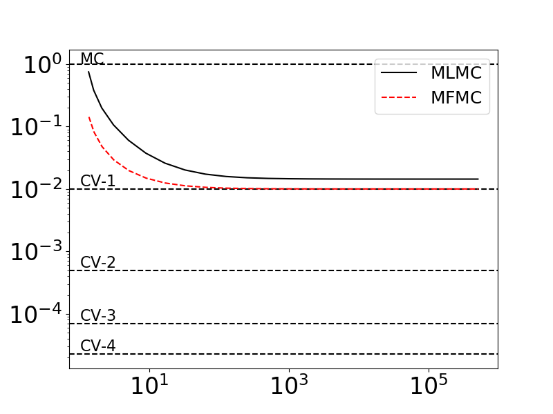
As you can see the MFMC (and MLMC) estimators only converge to the CV estimator that uses one low-fidelity model (CV-1). The associated allocation matrix are structured in such a way that only the model \(f_1\) is directly reducing the variance of \(Q_0\).

Improving MFMC optimization for small computational budgets

Typically MFMC solves a real values optimization to determine the optimal sample allocation that minimizes the estimator variance and then rounds the number of samples used to evaluate each model down to the nearest interger. This can be inefficient for very small computational budgets relative to the computational costs of evaluating each model. Consequently, an improved optimization algorithm (again only for estimating expectations) was introduced in [GGLZ2022].

References

[PWGSIAM2016] (1,2)

Peherstorfer, B., Willcox, K., Gunzburger, M., Optimal Model Management for Multifidelity Monte Carlo Estimation, 2016.

[GGLZ2022]

Gruber, A., Gunzburger, M., Ju, L. et al. A Multifidelity Monte Carlo Method for Realistic Computational Budgets. J Sci Comput 94, 2 (2023).