Note
Go to the end to download the full example code
Pilot Studies
The covariance of an ACV estimator depends on the covariance between the different model fidelities and other statistics, such as variance, depend on additional statistics properties of the model. In previous tutorials, we have assumed that thse statistics are available. However, in practice they must be estimated, because if we knew them we would not have to construct an MC estimator in the first place.
This tutorial presents how to use a pilot-study to compute the statistics needed to compute a MC-based estimator and compute its estimator covariance. We will focus on estimating the mean of a scalar model, but the procedures we describe here can easily be extended to estimation of other statistics such as variance. One simlpy must use a pilot study to compute the relevant quantities defined in Delta-Based Covariance Formulas For Approximate Control Variates
Computing an ACV estimator of a statistic requires computing \(\covar{\mat{Q}_0}{\mat{\Delta}}\text{ and} \covar{\mat{\Delta}}{\mat{\Delta}}\). These quantities in turn depend on the quantities in Delta-Based Covariance Formulas For Approximate Control Variates. For example, when estimating the mean we must compute
Typically, this is not available so we compute it with a pilot study. A pilot study evaluates all the available models at a small set of samples \(\rvset_\text{pilot}\) and computes the quantities necessary to construct an ACV estimator. For example when computing the mean we estimate
where
With an unlimited computational budget, we would drive \(N_\text{pilot}\to\infty\), however in practice we must use a finite number of samples which introduces an error in to an ACV estimator.
The following code quantities the impact of the size of the pilot sample on the accuracy of an ACV estimator. If the pilot size is too small the accuracy of the control variate coefficieints will be poor, however it is made larger, constructing the pilot study will eat into the computational budget used to construct the estimator which also degrades accuracy. These two concerns need to be balanced.
First setup the example
import numpy as np
import matplotlib.pyplot as plt

from pyapprox.benchmarks import setup_benchmark
from pyapprox.multifidelity.factory import get_estimator, multioutput_stats
from pyapprox.util.utilities import get_correlation_from_covariance
from pyapprox.util.visualization import mathrm_label

np.random.seed(1)
Now choose an estimator and optimally allocate it with oracle information, that is the exact model covariance. We will use MFMC because the optimal sample allocation can be obtained analytically which speeds up this tutorial. However other estimators can be used. Also note that if using MFMC to estimate variance or other stats its allocation it still uses the allocation that is only guaranteed to be optimal when estimating the mean. This is not true of any other estimator except MLMC.
target_cost = 100
est_name = "mfmc"
benchmark = setup_benchmark("polynomial_ensemble", nmodels=3)
nmodels = len(benchmark.funs)
costs = np.array([1, 0.1, 0.05])

stat_type = "mean"
# stat_type = "variance"

cov = benchmark.covariance
if stat_type == "mean":
    oracle_stats = benchmark.mean[0]
    oracle_stat_args = [cov]
else:
    oracle_stats = benchmark.covariance[0, 0]
    oracle_stat_args = [
        cov, benchmark.fun.covariance_of_centered_values_kronker_product()]

print(get_correlation_from_covariance(benchmark.covariance))

oracle_stat = multioutput_stats[stat_type](benchmark.nqoi)
oracle_stat.set_pilot_quantities(*oracle_stat_args)

oracle_est = get_estimator(est_name, oracle_stat, costs)
oracle_est.allocate_samples(target_cost)
print(oracle_est)
[[1.         0.99498744 0.97499604]
 [0.99498744 1.         0.99215674]
 [0.97499604 0.99215674 1.        ]]
MFMCEstimator(stat=MultiOutputMean, recursion_index=[0 1], criteria=-9.29 target_cost=99.6, ratios=[ 5.30769231 37.69230769], nsamples=[  26  164 1144])
Now lets look at the MSE of the ACV estimator when pilot samples of different sizes are used. First, create a function that computes an acv estimator for a single pilot study. We will then repeatedly call this function to compute the MSE.
Note, the function we define below can be replicated for most practical application of ACV estimation, but in such situations it sill only be called once.
from pyapprox.multifidelity.stats import MultiOutputMean
from pyapprox.multifidelity.factory import multioutput_stats
from functools import partial

def build_acv(funs, variable, target_cost, npilot_samples, adjust_cost=True,
              seed=1, stat_type="mean"):
    # run pilot study

    # Note must set random state if running with nprocs > 1
    random_states = [
        np.random.RandomState(seed*2*variable.num_vars()+ii)
        for ii in range(variable.num_vars())]
    # instead of np.random.seed(seed)
    pilot_samples = variable.rvs(npilot_samples, random_states=random_states)
    pilot_values_per_model = [fun(pilot_samples) for fun in funs]
    stat_class = multioutput_stats[stat_type]
    pilot_quantities = stat_class.compute_pilot_quantities(
        pilot_values_per_model)
    # print(get_correlation_from_covariance(pilot_cov))

    # optimize the ACV estimator
    stat = multioutput_stats[stat_type](benchmark.nqoi)
    stat.set_pilot_quantities(*pilot_quantities)
    est = get_estimator(est_name, stat, costs)
    # remaining_budget_after_pilot
    if adjust_cost:
        adjusted_target_cost = target_cost - (costs*npilot_samples).sum()
    else:
        adjusted_target_cost = target_cost
    # print(adjusted_target_cost)
    try:
        est.allocate_samples(adjusted_target_cost)
        # compute the ACV estimator
        random_states = [
            np.random.RandomState(
                seed*2*variable.num_vars()+variable.num_vars()+ii)
            for ii in range(variable.num_vars())]
        samples_per_model = est.generate_samples_per_model(
            partial(variable.rvs, random_states=random_states))
        values_per_model = [
            fun(samples) for fun, samples in zip(funs, samples_per_model)]
        est_stats = est(values_per_model)
        return est_stats
    except (RuntimeError, RuntimeWarning) as e:
        # sometimes MFMC will fail when used to find optimal solution
        # for variance because we cannot bound from below the number of
        # high-fidelity samples to be at least 2.
        # This causes the error
        # Degrees of freedom <= 0 for slice error occurs because
        # or
        # Rounding will cause nhf samples to be zero tensor
        # when nhf samples is below 1.
        print(e)
        return [np.inf]
Now define a function to compute the MSE. Note nprocs cannot be set > 1 unless all of this code is placed inside a function, e.g. called main, which is then run inside the following conditional
if __name__ == '__main__':
    main()
from multiprocessing import Pool
def compute_mse(build_acv, funs, variable, target_cost, npilot_samples,
                adjust_cost, ntrials, nprocs, exact_stats, stat_type):
    build = partial(
        build_acv, funs, variable, target_cost, npilot_samples, adjust_cost,
        stat_type=stat_type)
    if nprocs > 1:
        pool = Pool(nprocs)
        est_vals = pool.map(build, list(range(ntrials)))
        pool.close()
    else:
        est_vals = np.asarray([build(ii) for ii in range(ntrials)])

    # exclude failed MCMC runs
    est_vals = np.array(est_vals)[np.isfinite(est_vals)]
    # make sure random seed is getting set correctly on each processor
    assert np.unique(est_vals).shape[0] == len(est_vals)
    mse = ((est_vals-exact_stats)**2).mean()
    return mse
Ignoring the computational cost of the pilot study
Now we will build many realiaztions of the ACV estimator for each different samples size. We must ensure that the cost of the pilot study and the construction of the ACV estimator do not exceed the target cost.
np.random.seed(1)
ntrials = int(1e3)
mse_list = []
npilot_samples_list = [5, 10, 20, 40, 80, 160]
for npilot_samples in npilot_samples_list:
    print(npilot_samples)
    mse_list.append(compute_mse(
        build_acv, benchmark.funs, benchmark.variable, target_cost,
        npilot_samples, False, ntrials, 1, oracle_stats,
        stat_type))
    print(mse_list[-1])
5
Rounding will cause nhf samples to be zero tensor([2.0059e-01, 3.5647e+00, 1.9847e+03])
Rounding will cause nhf samples to be zero tensor([5.2019e-01, 8.5195e+00, 1.9625e+03])
Rounding will cause nhf samples to be zero tensor([8.5891e-01, 1.2316e+01, 1.9433e+03])
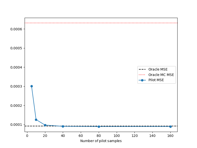
0.00030055376524214494
10
0.00012597668290734038
20
9.738350413654201e-05
40
9.059521503433804e-05
80
8.950838488655008e-05
160
8.98108769019937e-05
Now compare the MSE of the oracle ACV estimator which is just equal to its estimator variance, with the estimators constructed for different pilot samples sizes.
mc_est = get_estimator("mc", oracle_stat, costs)
mc_est.allocate_samples(target_cost)
mc_mse = mc_est._optimized_covariance[0, 0].item()

oracle_mse = oracle_est._optimized_covariance[0, 0].item()
ax = plt.subplots(1, 1, figsize=(8, 6))[1]
ax.axhline(y=oracle_mse, ls='--', color='k', label=mathrm_label("Oracle MSE"))
ax.axhline(y=mc_mse, ls=':', color='r', label=mathrm_label("Oracle MC MSE"))
ax.plot(npilot_samples_list, mse_list, '-o', label=mathrm_label("Pilot MSE"))
ax.set_xlabel(mathrm_label("Number of pilot samples"))
_ = ax.legend()
Accounting for the computational cost of the pilot study
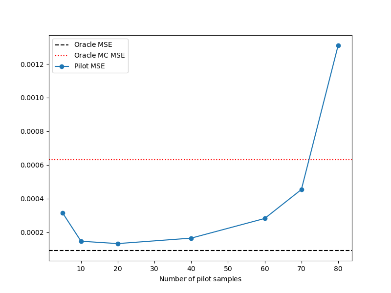
The previous study asssumed that the target cost of the estimator was not impacted by the computational cost of running the pilot study but this is not practical. Now lets plot the MSE vs the number of pilot samples keeping while ensuring that the cost of computing the pilot and the cost of constructing the estimator are always equal to the target cost
np.random.seed(1)
ntrials = int(1e3)
mse_list = []
target_cost = 100
# we must keep pilot cost below target cost
npilot_samples_list = [5, 10, 20, 40, 60, 70, 80]
for npilot_samples in npilot_samples_list:
    # The cost of evaluating all models once is np.sum(costs)
    pilot_cost = np.sum(costs)*npilot_samples
    print(npilot_samples)
    mse_list.append(compute_mse(
        build_acv, benchmark.funs, benchmark.variable, target_cost-pilot_cost,
        npilot_samples, False, ntrials, 1, oracle_stats,
        stat_type))
    print(mse_list[-1])

ax = plt.subplots(1, 1, figsize=(8, 6))[1]
ax.axhline(y=oracle_mse, ls='--', color='k', label=mathrm_label("Oracle MSE"))
ax.axhline(y=mc_mse, ls=':', color='r', label=mathrm_label("Oracle MC MSE"))
ax.plot(npilot_samples_list, mse_list, '-o', label=mathrm_label("Pilot MSE"))
ax.set_xlabel(mathrm_label("Number of pilot samples"))
_ = ax.legend()
5
Rounding will cause nhf samples to be zero tensor([1.8906e-01, 3.3597e+00, 1.8706e+03])
Rounding will cause nhf samples to be zero tensor([4.9028e-01, 8.0296e+00, 1.8496e+03])
Rounding will cause nhf samples to be zero tensor([8.0952e-01, 1.1608e+01, 1.8316e+03])
0.000314882320678576
10
0.00014706721463649233
20
0.0001330628522724495
40
0.00016543197783316097
60
0.00028222563377836794
70
0.00045427233226952914
80
0.001310297937485497
As you can see if the computational cost of the pilot study is a large fraction of the target cost then the MSE becomes very bad.
Estimating model costs
The pilot study is also used to approximate the model costs. Typically, we take the median run time of each model over the pilot samples
Estimating statistics other than the mean
Try setting stat_type=”variance”. What impact does it have on the MSE as a function of the number of pilot samples?
Total running time of the script: ( 0 minutes 20.988 seconds)