Two Model Control Variate Monte Carlo

This tutorial describes how to implement and deploy control variate Monte Carlo sampling to compute the statistics of the output of a high-fidelity model using a lower-fidelity model with a known mean. The information presented here builds upon the tutorial Monte Carlo Quadrature. We will focus on estimation of a single statistic for now, but control variates can be used to estiamte multiple statistics simultaneoulsy.

Let us introduce a model \(f_\kappa\) with known statistic \(Q_{\kappa}\). We can use this model to estimate the mean of \(f_{\alpha}\) via [LMWOR1982]

\[Q_{\alpha}^{\text{CV}}(\rvset_N) = Q_{\alpha}(\rvset_N) + \eta \left( Q_{\kappa}(\rvset_N) - Q_{\kappa} \right)\]

Here \(\eta\) is a free parameter which can be optimized to the reduce the variance of this so called control variate estimator, which is given by

\[\begin{split}\var{Q_{\alpha}^{\text{CV}}(\rvset_N)} &= \var{Q_{\alpha}(\rvset_N) + \eta \left( Q_{\kappa}(\rvset_N) - Q_{\kappa}\right)}\\ &=\var{Q_{\alpha}(\rvset_N)} + \eta^2\var{\left( Q_{\kappa}(\rvset_N) - Q_{\kappa}\right)}+ 2\eta\covar{Q_{\alpha}(\rvset_N)}{\left( Q_{\kappa}(\rvset_N) - Q_{\kappa}\right)}\\ &=\var{Q_{\alpha}(\rvset_N)}\left(1+\eta^2\frac{\var{\left( Q_{\kappa}(\rvset_N) - Q_{\kappa}\right)}}{\var{Q_{\alpha}(\rvset_N)}}+ 2\eta\frac{\covar{Q_{\alpha}(\rvset_N)}{\left( Q_{\kappa}(\rvset_N) - Q_{\kappa}\right)}}{\var{Q_{\alpha}(\rvset_N)}}\right).\end{split}\]

The first line follows from the variance of sums of random variables.

We can measure the change in MSE of the control variate estimator from the single model MC estimator, by looking at the ratio of the CVMC and MC estimator variances. This variance reduction ratio is

\[\gamma=\frac{\var{Q_{\alpha}^{\text{CV}}(\rvset_N)}}{\var{Q_{\alpha}(\rvset_N)}}=\left(1+\eta^2\frac{\var{\left( Q_{\kappa}(\rvset_N) - Q_{\kappa}\right)}}{\var{Q_{\alpha}(\rvset_N)}}+ 2\eta\frac{\covar{Q_{\alpha}(\rvset_N)}{\left( Q_{\kappa}(\rvset_N) - Q_{\kappa}\right)}}{\var{Q_{\alpha}(\rvset_N)}}\right)\]

and can be minimized by setting its gradient to zero and solving for \(\eta\), i.e.

\[\begin{split} \frac{d}{d\eta}\gamma &= 2\eta\frac{\var{\left( Q_{\kappa}(\rvset_N) - Q_{\kappa}\right)}}{\var{Q_{\alpha}(\rvset_N)}}+ 2\frac{\covar{Q_{\alpha}(\rvset_N)}{\left( Q_{\kappa}(\rvset_N) - Q_{\kappa}\right)}}{\var{Q_{\alpha}(\rvset_N)}} = 0\\ &\implies \eta\var{\left( Q_{\kappa}(\rvset_N) - Q_{\kappa}\right)}+ \covar{Q_{\alpha}(\rvset_N)}{\left( Q_{\kappa}(\rvset_N) - Q_{\kappa}\right)} = 0\\ &\implies \eta=-\frac{\covar{Q_{\alpha}(\rvset_N)}{\left( Q_{\kappa}(\rvset_N) - Q_{\kappa}\right)}}{\var{\left( Q_{\kappa}(\rvset_N) - Q_{\kappa}\right)}}\\ &\qquad\quad\;=-\frac{\covar{Q_{\alpha}(\rvset_N)}{Q_{\kappa}(\rvset_N)}}{\var{Q_{\kappa}(\rvset_N)}}\end{split}\]

With this choice

\[\begin{split}\gamma &= 1+\frac{\covar{Q_{\alpha}(\rvset_N)}{\left( Q_{\kappa}(\rvset_N) - Q_{\kappa}\right)}^2}{\var{\left( Q_{\kappa}(\rvset_N) - Q_{\kappa}\right)}^2}\frac{\var{\left( Q_{\kappa}(\rvset_N) - Q_{\kappa}\right)}}{\var{Q_{\alpha}(\rvset_N)}}\\&\qquad-2\frac{\covar{Q_{\alpha}(\rvset_N)}{\left( Q_{\kappa}(\rvset_N) - Q_{\kappa}\right)}}{\var{\left( Q_{\kappa}(\rvset_N) - Q_{\kappa}\right)}}\frac{\covar{Q_{\alpha}(\rvset_N)}{\left( Q_{\kappa}(\rvset_N) - Q_{\kappa}\right)}}{\var{Q_{\alpha}(\rvset_N)}}\\ &= 1+\frac{\covar{Q_{\alpha}(\rvset_N)}{\left( Q_{\kappa}(\rvset_N) - Q_{\kappa}\right)}^2}{\var{\left( Q_{\kappa}(\rvset_N) - Q_{\kappa}\right)}\var{Q_{\alpha}(\rvset_N)}}-2\frac{\covar{Q_{\alpha}(\rvset_N)}{\left( Q_{\kappa}(\rvset_N) - Q_{\kappa}\right)}^2}{\var{\left( Q_{\kappa}(\rvset_N) - Q_{\kappa}\right)}\var{Q_{\alpha}(\rvset_N)}}\\ &= 1-\corr{Q_{\alpha}(\rvset_N)}{\left( Q_{\kappa}(\rvset_N) - Q_{\kappa}\right)}^2\\ &= 1-\corr{Q_{\alpha}(\rvset_N)}{Q_{\kappa}(\rvset_N)}^2\end{split}\]

When estimating the mean we can use Equation to obtain

\[\begin{split}\eta &= -\frac{\covar{Q_{\alpha}(\rvset_N)}{Q_{\kappa}(\rvset_N)}}{\var{Q_{\kappa}(\rvset_N)}} \\ &= N^{-1}\frac{\covar{f_{\alpha}}{f_{\kappa}}}{N^{-1}\var{f_{\kappa}}}\\ &= \frac{\covar{f_{\alpha}}{f_{\kappa}}}{\var{f_{\kappa}}}\end{split}\]

which we can plug back into to \(\gamma\) to give

\[\begin{split}\gamma &= 1-\corr{Q_{\alpha}(\rvset_N)}{Q_{\kappa}(\rvset_N)}^2\\ &= 1-\corr{f_{\alpha}}{f_{\kappa}}^2\\\end{split}\]

and so

\[\var{Q_{\alpha}^{\text{CV}}(\rvset_N)} = \var{Q_{\alpha}(\rvset_N)}(1-\corr{f_{\alpha}}{f_{\kappa}}^2)\]

Thus, if two highly correlated models (one with a known mean) are available then we can drastically reduce the MSE of our estimate of the unknown mean. Similar reductions can be obtained for other statistics such as variance. But when estimating variance the estimator variance reduction ratio will no nolonger depend just on the correlation between the models but also higher order moments.

Again consider the tunable model ensemble. The correlation between the models \(f_0\) and \(f_1\) can be tuned by varying \(\theta_1\). For a given choice of theta lets compute a single relization of the CVMC estimate of \(Q_0=\mean{f_0}\)

First let us setup the problem and compute a single estimate using CVMC

import numpy as np
import matplotlib.pyplot as plt
from pyapprox.benchmarks import setup_benchmark

np.random.seed(1)
shifts = [.1, .2]
benchmark = setup_benchmark(
    "tunable_model_ensemble", theta1=np.pi/2*.95, shifts=shifts)
model = benchmark.fun

nsamples = int(1e2)
samples = benchmark.variable.rvs(nsamples)
values0 = model.m0(samples)
values1 = model.m1(samples)
cov = benchmark.covariance
eta = -cov[0, 1]/cov[0, 0]
#cov_mc = np.cov(values0,values1)
#eta_mc = -cov_mc[0,1]/cov_mc[0,0]
exact_integral_f0, exact_integral_f1 = 0, shifts[0]
cv_mean = values0.mean()+eta*(values1.mean()-exact_integral_f1)
print('MC difference squared =', (values0.mean()-exact_integral_f0)**2)
print('CVMC difference squared =', (cv_mean-exact_integral_f0)**2)

MC difference squared = 0.01473604359753749
CVMC difference squared = 5.954528881712521e-05

Now lets look at the statistical properties of the CVMC estimator

ntrials = 1000
means = np.empty((ntrials, 2))
for ii in range(ntrials):
    samples = benchmark.variable.rvs(nsamples)
    values0 = model.m0(samples)
    values1 = model.m1(samples)
    means[ii, 0] = values0.mean()
    means[ii, 1] = values0.mean()+eta*(values1.mean()-exact_integral_f1)

print("Theoretical variance reduction",
      1-cov[0, 1]**2/(cov[0, 0]*cov[1, 1]))
print("Achieved variance reduction",
      means[:, 1].var(axis=0)/means[:, 0].var(axis=0))

Theoretical variance reduction 0.055234554161570304
Achieved variance reduction 0.05749985629263281

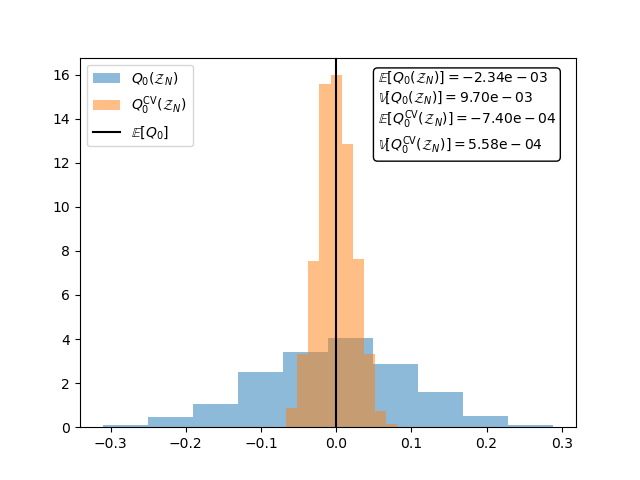
The following plot shows that unlike the MC estimator of. \(\mean{f_1}\) the CVMC estimator is unbiased and has a smaller variance.

fig,ax = plt.subplots()
textstr = '\n'.join(
    [r'$\mathbb{E}[Q_{0}(\mathcal{Z}_N)]=\mathrm{%.2e}$' % means[:, 0].mean(),
     r'$\mathbb{V}[Q_{0}(\mathcal{Z}_N)]=\mathrm{%.2e}$' % means[:, 0].var(),
     r'$\mathbb{E}[Q_{0}^\mathrm{CV}(\mathcal{Z}_N)]=\mathrm{%.2e}$' % (
         means[:, 1].mean()),
     r'$\mathbb{V}[Q_{0}^\mathrm{CV}(\mathcal{Z}_N)]=\mathrm{%.2e}$' % (
         means[:, 1].var())])
ax.hist(means[:, 0], bins=ntrials//100, density=True, alpha=0.5,
        label=r'$Q_{0}(\mathcal{Z}_N)$')
ax.hist(means[:, 1], bins=ntrials//100, density=True, alpha=0.5,
        label=r'$Q_{0}^\mathrm{CV}(\mathcal{Z}_N)$')
ax.axvline(x=0,c='k',label=r'$\mathbb{E}[Q_0]$')
props = {'boxstyle': 'round', 'facecolor': 'white', 'alpha': 1}
ax.text(0.6, 0.75, textstr,transform=ax.transAxes, bbox=props)
_ = ax.legend(loc='upper left')