Monte Carlo Quadrature

This tutorial describes how to use Monte Carlo sampling to compute the expectations of the output of a model $f(z):{\mathbb{R}}^D\to \mathbb{R}$ parameterized by a set of variables $z=[z_1,\dots ,z_D{]}^{\mathrm{\top }}$ with joint density given by $\rho (z):{\mathbb{R}}^d\to \mathbb{R}$. Specifically, our goal is to approximate the integral

$$Q={\int }_{\mathrm{\Gamma }}f(z)\rho (z)\text{d}z$$

using Monte Carlo quadrature applied to an approximation $f_{\alpha }$ of the function $f$, e.g. a representing a finite element approximation to the solution of a set of governing equations, where $\alpha$ is contols the accuracy of the approximation.

Monte Carlo quadrature approximates the integral

$$Q_{\alpha }={\int }_{\mathrm{\Gamma }}{f}_{\alpha }(z)\rho (z)\text{d}z\approx Q$$

by drawing $N$ random samples ${\mathcal{Z}}_N$ of $z$ from $\rho$ and evaluating the function at each of these samples to obtain the data pairs $\{(z^{(n)},f_{\alpha }^{(n)}){\}}_{n=1}^N$, where $f_{\alpha }^{(n)}=f_{\alpha }(z^{(n)})$ and computing

$$Q_{\alpha }({\mathcal{Z}}_N)=N^{-1}\sum _{n=1}^N{f}_{\alpha }^{(n)}$$

This estimate of the mean,is itself a random quantity, which we call an estimator, because its value depends on the ${\mathcal{Z}}_N$ realizations of the inputs ${\mathcal{Z}}_N$ used to compute $Q_{\alpha }({\mathcal{Z}}_N)$. Specifically, using two different sets ${\mathcal{Z}}_N$ will produce to different values.

To demonstrate this phenomenon, we will estimate the mean of a simple algebraic function $f_0$ which belongs to an ensemble of models

$$\begin{array}{rl}{f}_0(z)& =A_0(z_1^5\cos {\theta }_0+z_2^5\sin {\theta }_0),\\ f_1(z)& =A_1(z_1^3\cos {\theta }_1+z_2^3\sin {\theta }_1)+s_1,\\ f_2(z)& =A_2(z_1\cos {\theta }_2+z_2\sin {\theta }_2)+s_2\end{array}$$

where $z_1,z_2\sim \mathcal{U}(-1,1)$ and all $A$ and $\theta$ coefficients are real. We choose to set $A=\sqrt{11}$, $A_1=\sqrt{7}$ and $A_2=\sqrt{3}$ to obtain unitary variance for each model. The parameters $s_1,s_2$ control the bias between the models. Here we set $s_1=1/10,s_2=1/5$. Similarly we can change the correlation between the models in a systematic way (by varying ${\theta }_1$. We will levarage this later in the tutorial.

First setup the example

import numpy as np
import matplotlib.pyplot as plt

from pyapprox.benchmarks import setup_benchmark

np.random.seed(1)
shifts = [.1, .2]
benchmark = setup_benchmark(
    "tunable_model_ensemble", theta1=np.pi/2*.95, shifts=shifts)

Now define a function that computes MC estimates of the mean using different sample sets ${\mathcal{Z}}_N$ and plots the distribution the MC estimator $Q_{\alpha }({\mathcal{Z}}_N)$, computed from 1000 different sets, and the exact value of the mean $Q_{\alpha }$

def plot_estimator_histrogram(nsamples, model_id, ax):
    ntrials = 1000
    np.random.seed(1)
    means = np.empty((ntrials))
    model = benchmark.funs[model_id]
    for ii in range(ntrials):
        samples = benchmark.variable.rvs(nsamples)
        values = model(samples)
        means[ii] = values.mean()
    im = ax.hist(means, bins=ntrials//100, density=True, alpha=0.3,
                 label=r'$Q_{%d}(\mathcal{Z}_{%d})$' % (model_id, nsamples))[2]
    ax.axvline(x=benchmark.fun.get_means()[model_id], alpha=1,
               label=r'$Q_{%d}$' % model_id, c=im[0].get_facecolor())

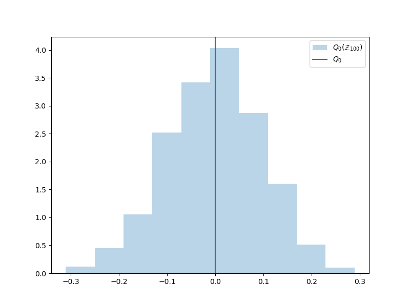
Now lets plot the historgram of the MC estimator $Q_0({\mathcal{Z}}_N)$ using $N=100$ samples

nsamples = int(1e2)
model_id = 0
ax = plt.subplots(1, 1, figsize=(8, 6))[1]
plot_estimator_histrogram(nsamples, model_id, ax)
_ = ax.legend()

The variability of the MC estimator as we change ${\mathcal{Z}}_N$ decreases as we increase $N$. To see this, plot the estimator historgram using $N=1000$ samples

model_id = 0
ax = plt.subplots(1, 1, figsize=(8, 6))[1]
nsamples = int(1e2)
plot_estimator_histrogram(nsamples, model_id, ax)
nsamples = int(1e3)
plot_estimator_histrogram(nsamples, model_id, ax)
_ = ax.legend()

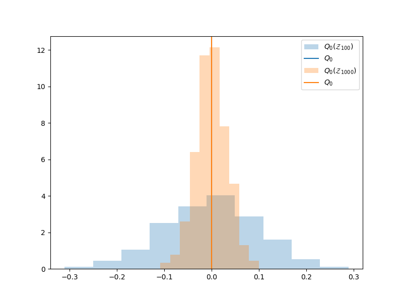
Regardless of the value of $N$ the estimator $Q_0({\mathcal{Z}}_N)$ is an unbiased estimate of $Q_0$, that is

$$\mathbb{E}[Q_0({\mathcal{Z}}_N)]-Q_0=0$$

Unfortunately, if the computational cost of evaluating a model is high, then one may not be able to make $N$ large using that model. Consequently, one will not be able to trust the MC estimate of the mean much because any one realization of the estimator, computed using a single sample set, may obtain a value that is very far from the truth. So often a cheaper less accurate model is used so that $N$ can be increased to reduce the variability of the estimator. The following compares the histograms of $Q_0({\mathcal{Z}}_{100})$ and $Q_1({\mathcal{Z}}_{1000})$ which uses the model $f_1$ which we assume is a cheap approximation of $f_0$

model_id = 0
ax = plt.subplots(1, 1, figsize=(8, 6))[1]
nsamples = int(1e2)
plot_estimator_histrogram(nsamples, model_id, ax)
model_id = 1
nsamples = int(1e3)
plot_estimator_histrogram(nsamples, model_id, ax)
_ = ax.legend()

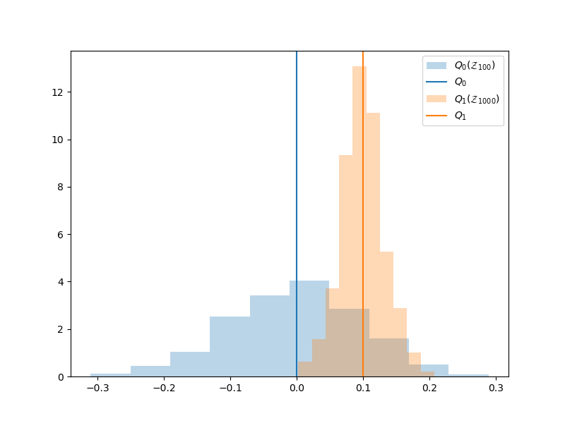
However, using an approximate model means that the MC estimator is no longer unbiased. The mean of the histogram of $Q_1({\mathcal{Z}}_{1000})$ is no longer the mean of $Q_0$

Letting $Q$ denote the true mean we want to estimate, e.g. $Q=Q_0$ in the example we have used so far, the mean squared error (MSE) is typically used to quantify the quality of a MC estimator. The MSE can be expressed as

$$\begin{array}{rl}\mathbb{E}\left[{(Q_{\alpha }({\mathcal{Z}}_N)-Q)}^2\right]& =\mathbb{E}\left[{(Q_{\alpha }({\mathcal{Z}}_N)-\mathbb{E}[Q_{\alpha }({\mathcal{Z}}_N)]+\mathbb{E}[Q_{\alpha }({\mathcal{Z}}_N)]-Q)}^2\right]\\ & =\mathbb{E}\left[{(Q_{\alpha }({\mathcal{Z}}_N)-\mathbb{E}[Q_{\alpha }({\mathcal{Z}}_N)])}^2\right]+\mathbb{E}\left[{(\mathbb{E}[Q_{\alpha }({\mathcal{Z}}_N)]-Q)}^2\right]\\ & +\mathbb{E}\left[2(Q_{\alpha }({\mathcal{Z}}_N)-\mathbb{E}[Q_{\alpha }({\mathcal{Z}}_N)])(\mathbb{E}[Q_{\alpha }({\mathcal{Z}}_N)]-Q)\right]\\ & =\mathbb{V}[Q_{\alpha }({\mathcal{Z}}_N)]+{(\mathbb{E}[Q_{\alpha }({\mathcal{Z}}_N)]-Q)}^2\\ & =\mathbb{V}[Q_{\alpha }({\mathcal{Z}}_N)]+{(Q_{\alpha }-Q)}^2\end{array}$$

where the expectation $\mathbb{E}$ and variance $\mathbb{V}$ are taken over different realization of the sample set ${\mathcal{Z}}_N$, we used that $\mathbb{E}\left[(Q_{\alpha }({\mathcal{Z}}_N)-\mathbb{E}[Q_{\alpha }({\mathcal{Z}}_N)])\right]=0$ so the third term on the second line is zero, and we used $\mathbb{E}[Q_{\alpha }({\mathcal{Z}}_N)]=Q_{\alpha }$ to get the final equality.

Now using the well known result that for random variable $X_n$

$$\mathbb{V}\left[\sum _{n=1}^N{X}_n\right]=\sum _{n=1}^N\mathbb{V}\left[X_n\right]+\sum _{n\ne p}\mathbb{C}\text{ov}[X_n,X_p]$$

and the result for a scalar $a$

$$\mathbb{V}\left[a{X}_n\right]=a^2\mathbb{V}\left[X_n\right]$$

yields

$$\mathbb{V}[Q_{\alpha }({\mathcal{Z}}_N)]=\mathbb{V}\left[N^{-1}\sum _{n=1}^N{f}_{\alpha }^{(n)}\right]=N^{-2}\sum _{n=1}^N\mathbb{V}\left[f_{\alpha }^{(n)}\right]=N^{-1}\mathbb{V}\left[f_{\alpha }\right]$$

where $\mathbb{C}\text{ov}[f^{(n)},f^{(p)}]=0,n\ne p$ because the samples are drawn independently.

Finally, substituting $\mathbb{V}[Q_{\alpha }({\mathcal{Z}}_N)]$ into the expression for MSE yields

$$\mathbb{E}\left[{(Q_{\alpha }({\mathcal{Z}}_N)-\mathbb{E}\left[Q\right])}^2\right]=\underset{I}{\underbrace{N^{-1}\mathbb{V}\left[f_{\alpha }\right]}}+\underset{II}{\underbrace{{(Q_{\alpha }-Q)}^2}}$$

From this expression we can see that the MSE can be decomposed into two terms; a so called stochastic error (I) and a deterministic bias (II). The first term is the variance of the Monte Carlo estimator which comes from using a finite number of samples. The second term is due to using an approximation of $f_0$. These two errors should be balanced, however in the vast majority of all MC analyses a single model $f_{\alpha }$ is used and the choice of $\alpha$, e.g. mesh resolution, is made a priori without much concern for the balancing bias and variance.

Video

Click on the image below to view a video tutorial on Monte Carlo quadrature