Note
Go to the end to download the full example code
Multifidelity Gaussian processes
This tutorial describes how to implement and deploy multi-level Gaussian processes built using the output of a high-fidelity model and evaluations of a set of lower-fidelity models of lower accuracy and cost [KOB2000]. This tutorial assumes understanding of the concepts in Gaussian processes
Multilevel GPs assume that all the available models \(\{f_m\}_{m=1}^M\) can be ordered into a hierarchy of increasing cost and accuracy, where \(m=1\) denotes the lowest fidelity model and \(m=M\) denotes the hightest-fidelity model. We model the output \(y_m\) from the \(m\)-th level code as \(y_m = f_m(\rv)\) and assume the models satisfy the hierarchical relationship
with \(f_1(\rv)=\delta_1(\rv)\). We assume that the prior distributions on \(\delta_m(\cdot)\sim\mathcal{N}(0, C_m(\cdot,\cdot))\) are independent.
Just like traditional GPs the posterior mean and variance of the multi-fidelity GP are given by
where \(C(\mathcal{Z}, \mathcal{Z})\) is the prior covariance evaluated at the training data \(\mathcal{Z}\).
The difference comes from the definitions of the prior covariance \(C\) and the vector \(t(\rv)\).
Two models
Given data \(\mathcal{Z}=[\mathcal{Z}_1, \mathcal{Z}_2]\) from two models of differing fidelity, the data covariance of the multi-fidelity GP consisting of two models can be expressed in block form
The upper-diagonal block is given by
The lower-diagonal block is given by
Where on the second last line we used that \(\delta_1\) and \(\delta_2\) are independent.
The upper-right block is given by
and \(\covar{f_2(\mathcal{Z}_2)}{f_1(\mathcal{Z}_1)}=\covar{f_1(\mathcal{Z}_2)}{f_2(\mathcal{Z}_2)}^\top.\)
Combining yields
In this tutorial we assume \(\rho_m\) are scalars. However PyApprox supports polynomial versions \(\rho_m(\rv)\). The above formulas must be slightly modified in this case.
Similary we have
where
M models
The diagonal covariance blocks of the prior covariance \(C\) for \(m>1\) satisfy
The off-diagonal covariance blocks for \(m<n\) satisfy
For example, the covariance matrix for \(M=3\) models is
and \(t_m\) is the mth row of \(C\) that replaces the first argument of each covariance kernel with \(\rv\), for example
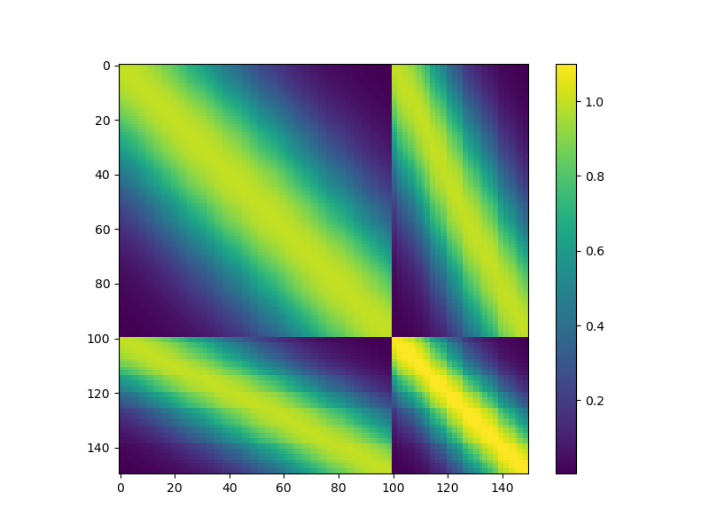
Now lets plot the structure of the multi-fidelity covariance matrix when using two models and scalar scaling \(\rho\). The blocks correspond to the four blocks of the two model data covariance matrix.
from scipy import stats
import numpy as np
import matplotlib.pyplot as plt
from pyapprox.variables.joint import IndependentMarginalsVariable
from pyapprox.surrogates.gaussianprocess.multilevel import (
    GreedyMultifidelityIntegratedVarianceSampler, MultifidelityGaussianProcess,
    GaussianProcess, SequentialMultifidelityGaussianProcess)
from pyapprox.surrogates.gaussianprocess.kernels import (
    RBF, MultifidelityPeerKernel, MonomialScaling)
from pyapprox.surrogates.integrate import integrate

np.random.seed(1)
nvars = 1
variable = IndependentMarginalsVariable(
            [stats.uniform(0, 1) for ii in range(nvars)])

nmodels = 2
kernels = [RBF for nn in range(nmodels)]
sigma = [1, 0.1]
length_scale = np.hstack([np.full(nvars, 0.3)]*nmodels)

rho = [1.0]
degree = 0
kernel_scalings = [
    MonomialScaling(nvars, degree) for nn in range(nmodels-1)]
kernel = MultifidelityPeerKernel(
    nvars, kernels, kernel_scalings, length_scale=length_scale,
    length_scale_bounds=(1e-10, 1), rho=rho,
    rho_bounds=(1e-3, 1), sigma=sigma,
    sigma_bounds=(1e-3, 2))

# sort for plotting covariance matrices
nsamples_per_model = [100, 50]
train_samples = [
    np.sort(integrate("quasimontecarlo", variable,
                      nsamples=nsamples_per_model[nn],
                      startindex=1000*nn+1)[0], axis=1)
    for nn in range(nmodels)]

ax = plt.subplots(1, 1, figsize=(1*8, 6))[1]
kernel.set_nsamples_per_model(nsamples_per_model)
Kmat = kernel(np.hstack(train_samples).T)
im = ax.imshow(Kmat)
plt.colorbar(im, ax=ax)
<matplotlib.colorbar.Colorbar object at 0x16b35e6e0>
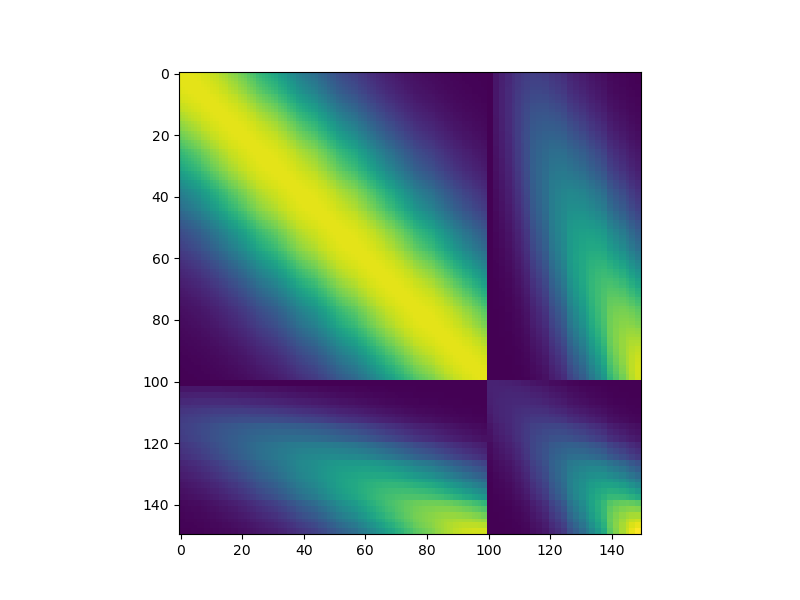
Now lets plot the structure of the multi-fidelity covariance matrix when using two models a linear polynomial scaling \(\rho(x)=a+bx\). In comparison to a scalar scaling the correlation between the low and high-fidelity models changes as a function of the input \(\rv\).
ax = plt.subplots(1, 1, figsize=(1*8, 6))[1]
rho_2 = [0., 1.0]  # [a, b]
kernel_scalings_2 = [
    MonomialScaling(nvars, 1) for nn in range(nmodels-1)]
kernel_2 = MultifidelityPeerKernel(
    nvars, kernels, kernel_scalings_2, length_scale=length_scale,
    length_scale_bounds=(1e-10, 1), rho=rho_2,
    rho_bounds=(1e-3, 1), sigma=sigma,
    sigma_bounds=(1e-3, 1))
kernel_2.set_nsamples_per_model(nsamples_per_model)
Kmat2 = kernel_2(np.hstack(train_samples).T)
im = ax.imshow(Kmat2)
Now lets define two functions with multilevel structure
def scale(x, rho, kk):
    if degree == 0:
        return rho[kk]
    if x.shape[0] == 1:
        return rho[2*kk] + x.T*rho[2*kk+1]
    return rho[3*kk] + x[:1].T*rho[3*kk+1]+x[1:2].T*rho[3*kk+2]


def f0(x):
    # y = x.sum(axis=0)[:, None]
    y = x[0:1].T
    return ((y*3-1)**2+1)*np.sin((y*10-2))/5


def f1(x):
    # y = x.sum(axis=0)[:, None]
    y = x[0:1].T
    return scale(x, rho, 0)*f0(x)+((y-0.5))/2
Now build a GP with 8 samples from the low-fidelity model and four samples from the high-fidelity model
nsamples_per_model = [8, 4]
train_samples = [
    np.sort(integrate("quasimontecarlo", variable,
                      nsamples=nsamples_per_model[nn],
                      startindex=1000*nn+1)[0], axis=1)
    for nn in range(nmodels)]
true_rho = np.full((nmodels-1)*degree+1, 0.9)
models = [f0, f1]
train_values = [f(x) for f, x in zip(models, train_samples)]

gp = MultifidelityGaussianProcess(kernel, n_restarts_optimizer=20)
gp.set_data(train_samples, train_values)
gp.fit()
prior_kwargs = {"color": "gray", "alpha": 0.3}
ax = plt.subplots(1, 1, figsize=(8, 6))[1]
ax.plot(train_samples[0][0], train_values[0], 'ko')
ax.plot(train_samples[1][0], train_values[1], 'rs')
xx = np.linspace(0, 1, 101)[None, :]
ax.plot(xx[0], models[0](xx), 'k-', label=r"$f_0$")
ax.plot(xx[0], models[1](xx), 'r-', label=r"$f_1$")
gp.plot_1d(101, [0, 1], plt_kwargs={"ls": "--", "label": "MF2", "c": "b"},
           ax=ax, fill_kwargs={"color": "b", "alpha": 0.3})
gp.plot_1d(101, [0, 1], plt_kwargs={"ls": ":", "label": "MF1", "c": "g"},
           ax=ax, model_eval_id=0)
_ = ax.legend()
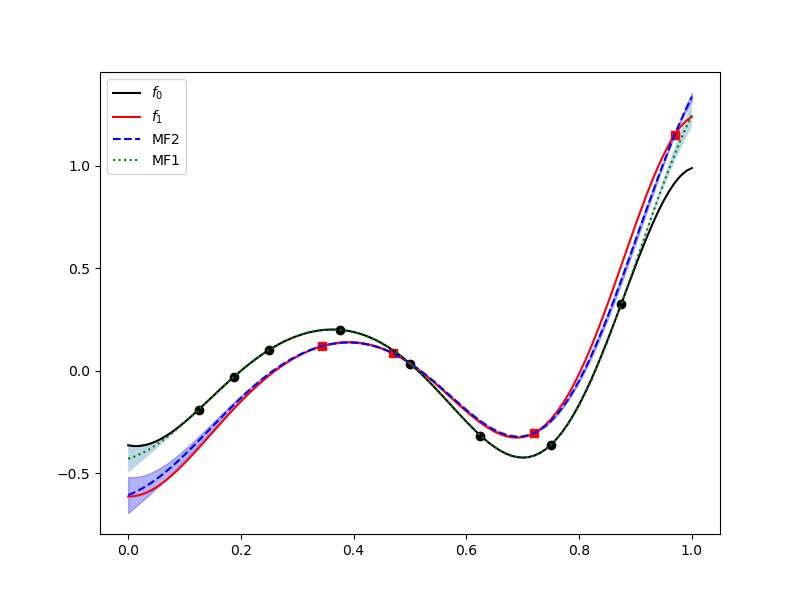
The low-fidelity model is very well approximated and the high-fidelity is very good even away from the high-fidelity training data. The low-fidelity data is being used to extrapolate.
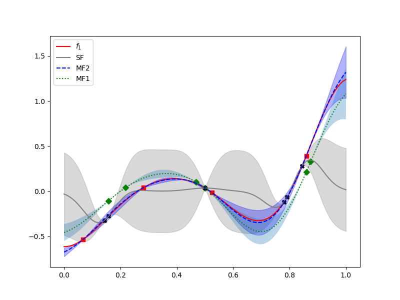
Now lets compare the multi-fidelity GP to a single fidelity GP built using only the high-fidelity data
sf_kernel = 1.0*RBF(length_scale[0], (1e-3, 1))
sf_gp = GaussianProcess(sf_kernel)
sf_gp.fit(train_samples[1], train_values[1])

ax = plt.subplots(1, 1, figsize=(8, 6))[1]
ax.plot(xx[0], models[1](xx), 'r-', label=r"$f_1$")
ax.plot(train_samples[1][0], train_values[1], 'rs')
ax.plot(train_samples[0][0], train_values[0], 'ko')
sf_gp.plot_1d(101, [0, 1], plt_kwargs={"label": "SF", "c": "gray"}, ax=ax,
              fill_kwargs={"color": "gray", "alpha": 0.3})
gp.plot_1d(101, [0, 1], plt_kwargs={"ls": "--", "label": "MF2", "c": "b"},
           ax=ax, fill_kwargs={"color": "b", "alpha": 0.3})
gp.plot_1d(101, [0, 1], plt_kwargs={"ls": ":", "label": "MF1", "c": "g"},
           ax=ax, model_eval_id=0)
_ = ax.legend()
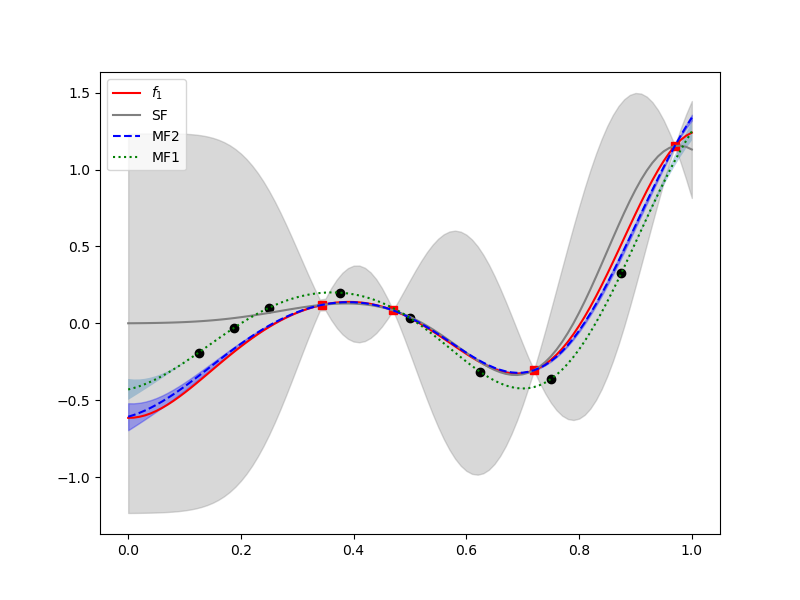
The single fidelity approximation of the high-fidelity model is much worse than the multi-fidelity approximation.
Sequential Construction
The computational cost of the multi-level GP presented grows cubically with the number of model evaluations \(N_m\) for all models, that is the number of operations is
When the training data is nested, e.g. \(\mathcal{Z_m}\subseteq \mathcal{Z}_{m+1}\) and noiseless, the algorithm in [LGIJUQ2014] can be used to construct a MF GP in
operations.
Another popular approach used to build MF GPs with either nested or unnested noisy data is to construct a single fidelity GP of the lowest model, then fix that GP and consruct a GP of the difference. This sequential algorithm is also much cheaper than the algorithm presented here, but the mean of the sequentially constructed GP is often less accurate and the posterior variance over- or under-estimated.
The following plot compares a sequential multi-level GP with the exact co-kriging on the toy problem introduced earlier.
sml_kernels = [
    RBF(length_scale=0.1, length_scale_bounds=(1e-10, 1))
    for ii in range(nmodels)]
sml_gp = SequentialMultifidelityGaussianProcess(
    sml_kernels, n_restarts_optimizer=20, default_rho=[1.0])
sml_gp.set_data(train_samples, train_values)
sml_gp.fit()

ax = plt.subplots(1, 1, figsize=(8, 6))[1]
ax.plot(xx[0], models[0](xx), 'k-', label=r"$f_0$")
ax.plot(xx[0], models[1](xx), 'r-', label=r"$f_1$")
ax.plot(train_samples[1][0], train_values[1], 'rs')
gp.plot_1d(101, [0, 1], plt_kwargs={"ls": "--", "label": "Co-kriging", "c": "b"},
           ax=ax, fill_kwargs={"color": "b", "alpha": 0.3})
_ = sml_gp.plot_1d(101, [0, 1],
                   plt_kwargs={"ls": "--", "label": "Sequential", "c": "g"},
                   ax=ax, fill_kwargs={"color": "g", "alpha": 0.3})
Experimental design
As with single fidelity GPs the location of the training data significantly impacts the accuracy of a multi-fidelity GP. The remainder of this tutorial discusses xtensions of the experimental design methods used for single-fidelity GPs in Gaussian processes.
The following code demonstrates the additional complexity faced when desigining experimental designs for multi-fidelity GPs, specifically one must not only choose what input to sample but also what model to sample.
ax = plt.subplots(1, 1, figsize=(8, 6))[1]
kernel = MultifidelityPeerKernel(
    nvars, kernels, kernel_scalings, length_scale=length_scale,
    length_scale_bounds="fixed", rho=rho,
    rho_bounds="fixed", sigma=sigma,
    sigma_bounds="fixed")

# build GP using only one low-fidelity data point. The values of the function
# do not matter as we are just going to plot the pointwise variance of the GP.
gp_2 = MultifidelityGaussianProcess(kernel)
gp_2.set_data([np.full((nvars, 1), 0.5), np.empty((nvars, 0))],
              [np.zeros((1, 1)), np.empty((0, 1))])
gp_2.fit()

# plot the variance of the multi-fidelity GP approximation of the
# high-fidelity model
gp_2.plot_1d(101, [0, 1],
             plt_kwargs={"ls": "--", "label": "1 LF data", "c": "gray"},
             ax=ax, fill_kwargs={"color": "g", "alpha": 0.3})
ax.plot(0.5, 0, 'rs', ms=15)

# build GP using only one high-fidelity data point
gp_2.set_data([np.empty((nvars, 0)), np.full((nvars, 1), 0.5)],
              [np.empty((0, 1)), np.zeros((1, 1))])
gp_2.fit()
gp_2.plot_1d(101, [0, 1],
             plt_kwargs={"ls": "--", "label": "1 HF data", "c": "b"},
             ax=ax, fill_kwargs={"color": "b", "alpha": 0.3})
ax.plot(0.5, 0, 'ko')
_ = ax.legend()
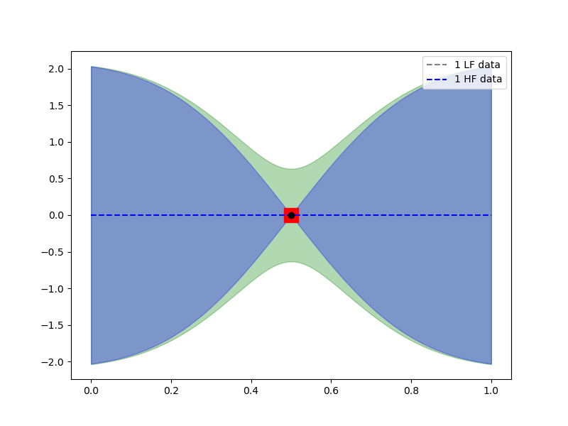
As expected the high-fidelity data point reduces the high-fidelity GP variance the most.
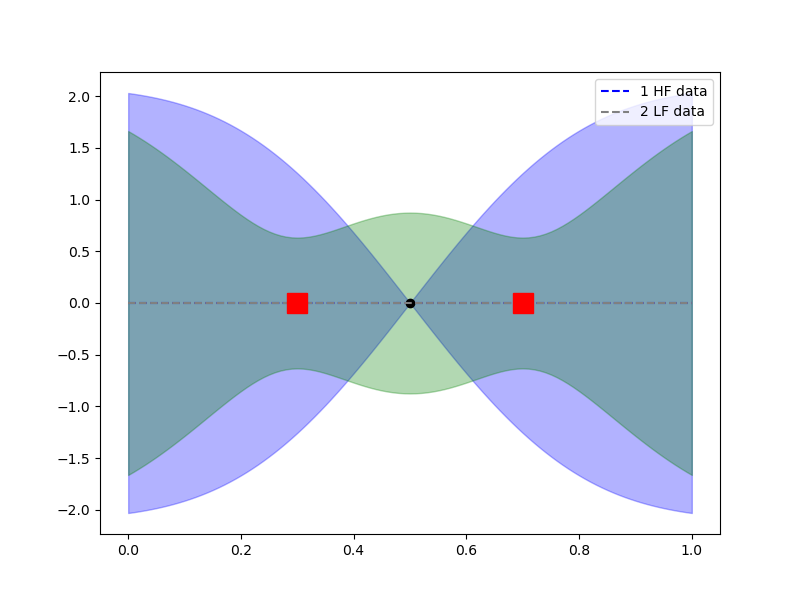
The following shows that two low-fidelity points may produce smaller variance than a single high-fidelity point.
ax = plt.subplots(1, 1, figsize=(8, 6))[1]

# plot one point high-fidelity GP against two low-fidelity points
gp_2.plot_1d(101, [0, 1],
             plt_kwargs={"ls": "--", "label": "1 HF data", "c": "b"},
             ax=ax, fill_kwargs={"color": "b", "alpha": 0.3})
ax.plot(0.5, 0, 'ko')

# build GP using twp low-fidelity data points.
gp_2.set_data([np.array([[0.3, 0.7]]), np.empty((nvars, 0))],
              [np.zeros((2, 1)), np.empty((0, 1))])
gp_2.fit()
gp_2.plot_1d(101, [0, 1],
             plt_kwargs={"ls": "--", "label": "2 LF data", "c": "gray"},
             ax=ax, fill_kwargs={"color": "g", "alpha": 0.3})
ax.plot([0.3, 0.7], [0, 0], 'rs', ms=15)
_ = ax.legend()
Analagous to single-fidelity GPs we will now use integrated variance to produce good experimental designs. Two model, multi-fidelity, integrated variance designs, as they are often called, find a set of samples \(\mathcal{Z}\subset\Omega\subset\rvdom\) from a set of candidate samples \(\Omega=\Omega_1\cup\Omega_2\) by greedily selecting a new point \(\rv^{(n+1)}\) to add to an existing set \(\mathcal{Z}_n\) according to
Here \(\Omega_m\) denotes the candidate samples for the mth model, \(W(\rv)\) is the cost of evaluating the candidate which is typically constant for all inputs for a given model, but different between models.
Now generate a sample set
nquad_samples = 1000
model_costs = np.array([1, 3])
ncandidate_samples_per_model = 101
sampler = GreedyMultifidelityIntegratedVarianceSampler(
    nmodels, nvars, nquad_samples, ncandidate_samples_per_model,
    variable.rvs, variable, econ=True,
    compute_cond_nums=False, nugget=0, model_costs=model_costs)

integrate_args = ["tensorproduct", variable]
integrate_kwargs = {"rule": "gauss", "levels": 100}
sampler.set_kernel(kernel, *integrate_args, **integrate_kwargs)

nsamples = 10
samples = sampler(nsamples)[0]
Now fit a GP with the selected samples
train_samples = np.split(
    samples, np.cumsum(sampler.nsamples_per_model).astype(int)[:-1],
    axis=1)
nsamples_per_model = np.array([s.shape[1] for s in train_samples])
costs = nsamples_per_model*model_costs
total_cost = costs.sum()
print("NSAMPLES", nsamples_per_model)
print("TOTAL COST", total_cost)
train_values = [f(x) for f, x in zip(models, train_samples)]
gp.set_data(train_samples, train_values)
gp.fit()
NSAMPLES [6 4]
TOTAL COST 18
Now build a single-fidelity GP using IVAR.
from pyapprox.surrogates.gaussianprocess.gaussian_process import (
    GreedyIntegratedVarianceSampler)
sf_sampler = GreedyIntegratedVarianceSampler(
    nvars, 2000, 1000, variable.rvs,
    variable, use_gauss_quadrature=True, econ=True,
    compute_cond_nums=False, nugget=0)
sf_sampler.set_kernel(sf_kernel)
nsf_train_samples = int(total_cost//model_costs[1])
print("NSAMPLES SF", nsf_train_samples)
sf_train_samples = sf_sampler(nsf_train_samples)[0]
sf_kernel = 1.0*RBF(length_scale[0], (1e-3, 1))
sf_gp = GaussianProcess(sf_kernel)
sf_train_values = models[1](sf_train_samples)
_ = sf_gp.fit(sf_train_samples, sf_train_values)
NSAMPLES SF 6
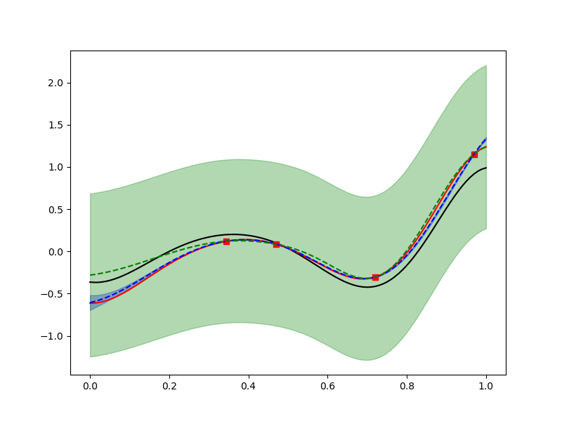
Compare the multi- and single-fidelity GPs.
ax = plt.subplots(1, 1, figsize=(8, 6))[1]
ax.plot(xx[0], models[1](xx), 'r-', label=r"$f_1$")
ax.plot(train_samples[0][0], train_values[0], 'gD')
ax.plot(train_samples[1][0], train_values[1], 'rs')
ax.plot(sf_train_samples[0], sf_train_values, 'kX')
sf_gp.plot_1d(101, [0, 1], plt_kwargs={"label": "SF", "c": "gray"}, ax=ax,
              fill_kwargs={"color": "gray", "alpha": 0.3})
gp.plot_1d(101, [0, 1], plt_kwargs={"ls": "--", "label": "MF2", "c": "b"},
           ax=ax, fill_kwargs={"color": "b", "alpha": 0.3})
gp.plot_1d(101, [0, 1], plt_kwargs={"ls": ":", "label": "MF1", "c": "g"},
           ax=ax, model_eval_id=0)
_ = ax.legend()
The multi-fidelity GP is again clearly superior.
Note the selected samples depend on hyperparameter values, change the hyper-parameters and see how the design changes. The relative cost of evaluating each model also impacts the design. For fixed hyper-parameters a larger ratio will typically result in more low-fidelity samples.
Remarks
Some approaches train the GPs of each sequentially, that is train a GP of the lowest-fidelity model. The lowest-fidelity GP is then fixed and data from the next lowest fidelity model is then used to train the GP associated with that data, and so on. However this approach typically produces less accurate approximations (GP means) and does not provide a way to estimate the correct posterior uncertainty of the multilevel GP.
Multifidelity Deep Gaussian Processes
The aforementioned algorithms assumed that the hierarchy of models are linearly related. However, for some model ensembles this may be inefficient and a nonlinear relationship may be more appropriate, e.g.
where \(g\) is a nonlinear function. Setting \(g\) to be Gaussian process leads to multi-fidelity deep Gaussian processes [KPDL2019], [PRDLK2017].
The following figures (generated using Emukit [EMUKIT]) demonstrate that the nonlinear formulation works better for the bi-fidelity model enesmble
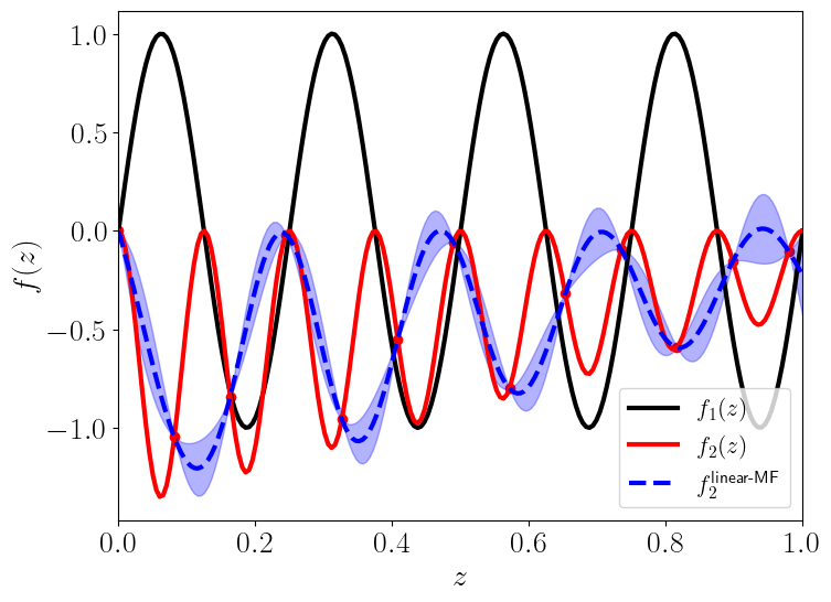
Linear MF GP |
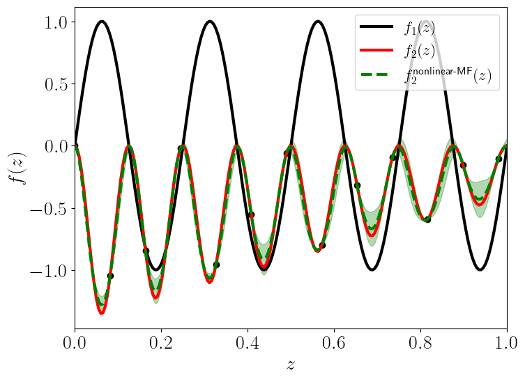
Nonlinear MF GP |
The following plots the correlations between the models used previously in this tutorial with the non-linear ensemble used here
axs = plt.subplots(1, 2, figsize=(2*8, 6))[1]
nonlinear_models = [lambda xx: np.sin(np.pi*8*xx.T),
                    lambda xx: (xx.T-np.sqrt(2))*np.sin(np.pi*8*xx.T)**2]
axs[0].plot(models[0](xx), models[1](xx))
axs[1].plot(nonlinear_models[0](xx), nonlinear_models[1](xx))
# axs[0].legend(['HF-LF Correlation'])
# axs[1].legend(['HF-LF Correlation'])
axs[0].set_xlabel(r'$f_1(z)$')
axs[0].set_ylabel(r'$f_2(z)$')
axs[1].set_xlabel(r'$f_1^{\mathrm{NL}}(z)$')
_ = axs[1].set_ylabel(r'$f_2^{\mathrm{NL}}(z)$')
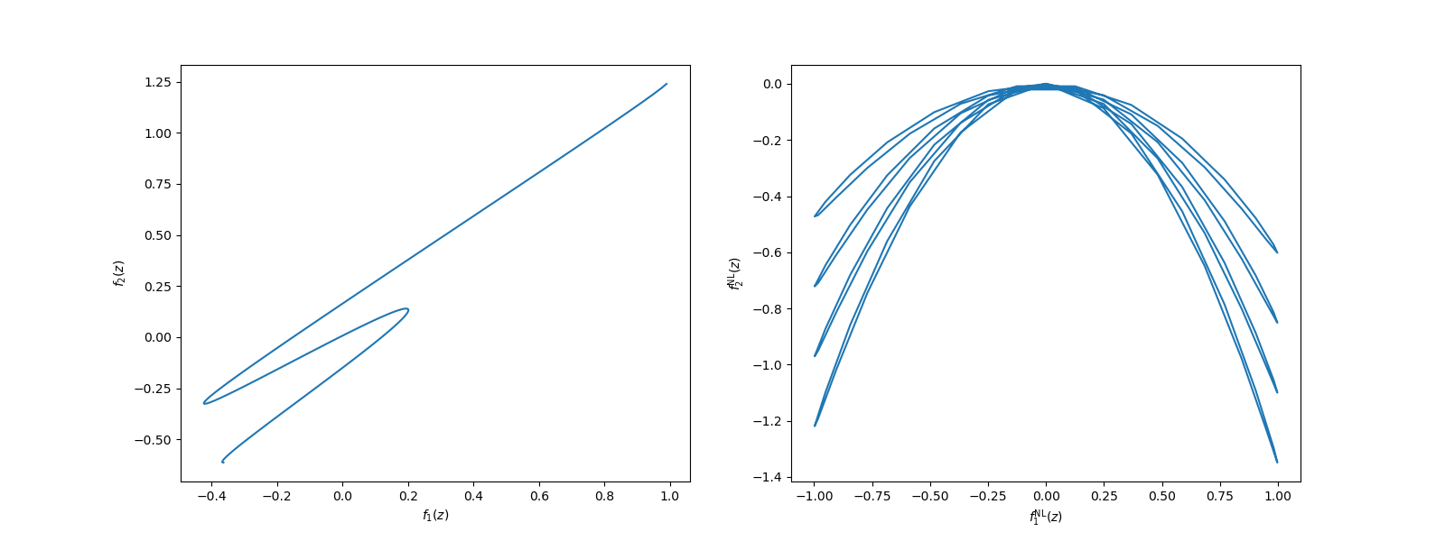
No exact statements can be made about a problem from such plots, however according to [PRDLK2017], the additional complexity of the models with the non-linear relationship often indicates that a linear MF GP will perform poorly.
References
Total running time of the script: ( 0 minutes 3.811 seconds)