Tensor-product Interpolation

Many simulation models are extremely computationally expensive such that adequately understanding their behaviour and quantifying uncertainty can be computationally intractable for any of the aforementioned techniques. Various methods have been developed to produce surrogates of the model response to uncertain parameters, the most efficient are goal-oriented in nature and target very specific uncertainty measures.

Generally speaking surrogates are built using a “small” number of model simulations and are then substituted in place of the expensive simulation models in future analysis. Some of the most popular surrogate types include polynomial chaos expansions (PCE) [XKSISC2002], Gaussian processes (GP) [RWMIT2006], and sparse grids (SG) [BGAN2004].

Reduced order models (e.g. [SFIJNME2017]) can also be used to construct surrogates and have been applied successfully for UQ on many applications. These methods do not construct response surface approximations, but rather solve the governing equations on a reduced basis. PyApprox does not currently implement reduced order modeling, however the modeling analyis tools found in PyApprox can easily be applied to assess or design systems based on reduced order models.

The use of surrogates for model analysis consists of two phases: (1) construction; and (2) post-processing.

Construction

In this section we show how to construct a surrogate using tensor-product Lagrange interpolation.

Tensor-product Lagrange interpolation

Let \(\hat{f}_{\boldsymbol{\alpha},\boldsymbol{\beta}}(\mathbf{z})\) be an M-point tensor-product interpolant of the function \(\hat{f}_{\boldsymbol{\alpha}}\). This interpolant is a weighted linear combination of tensor-product of univariate Lagrange polynomials

\[\phi_{i,j}(z_i) = \prod_{k=1,k\neq j}^{m_{\beta_i}}\frac{z_i-z_i^{(k)}}{z_i^{(j)}-z_i^{(k)}}, \quad i\in[d],\]

defined on a set of univariate points \(z_{i}^{(j)},j\in[m_{\beta_i}]\) Specifically the multivariate interpolant is given by

\[\hat{f}_{\boldsymbol{\alpha},\boldsymbol{\beta}}(\mathbf{z}) = \sum_{\boldsymbol{j}\le\boldsymbol{\beta}} \hat{f}_{\boldsymbol{\alpha}}(\mathbf{z}^{(\boldsymbol{j})})\prod_{i\in[d]}\phi_{i,j_i}(z_i).\]

The partial ordering \(\boldsymbol{j}\le\boldsymbol{\beta}\) is true if all the component wise conditions are true.

Constructing the interpolant requires evaluating the function \(\hat{f}_{\boldsymbol{\alpha}}\) on the grid of points

\[\mathcal{Z}_{\boldsymbol{\beta}} = \bigotimes_{i=1}^d \mathcal{Z}_{\beta_i}^i=\begin{bmatrix}\mathbf{z}^{(1)} & \cdots&\mathbf{z}^{(M_{\boldsymbol{\beta}})}\end{bmatrix}\in\mathbb{R}^{d\times M_{\boldsymbol{\beta}}}\]

We denote the resulting function evaluations by

\[\mathcal{F}_{\boldsymbol{\alpha},\boldsymbol{\beta}}=\hat{f}_{\boldsymbol{\alpha}}(\mathcal{Z}_{\boldsymbol{\beta}})=\begin{bmatrix}\hat{f}_{\boldsymbol{\alpha}}(\mathbf{z}^{(1)}) \quad \cdots\quad \hat{f}_{\boldsymbol{\alpha}}(\mathbf{z}^{(M_{\boldsymbol{\beta}})})\end{bmatrix}^T\in\mathbb{R}^{M_{\boldsymbol{\beta}}\times q},\]

where the number of points in the grid is \(M_{\boldsymbol{\beta}}=\prod_{i\in[d]} m_{\beta_i}\)

It is often reasonable to assume that, for any \(\mathbf{z}\), the cost of each simulation is constant for a given \(\boldsymbol{\alpha}\). So letting \(W_{\boldsymbol{\alpha}}\) denote the cost of a single simulation, we can write the total cost of evaluating the interpolant \(W_{\boldsymbol{\alpha},\boldsymbol{\beta}}=W_{\boldsymbol{\alpha}} M_{\boldsymbol{\beta}}\). Here we have assumed that the computational effort to compute the interpolant once data has been obtained is negligible, which is true for sufficiently expensive models \(\hat{f}_{\boldsymbol{\alpha}}\). Here we will use the nested Clenshaw-Curtis points

\[z_{i}^{(j)}=\cos\left(\frac{(j-1)\pi}{m_{\beta_i}-1}\right),\qquad j=1,\ldots,m_{\beta_i}\]

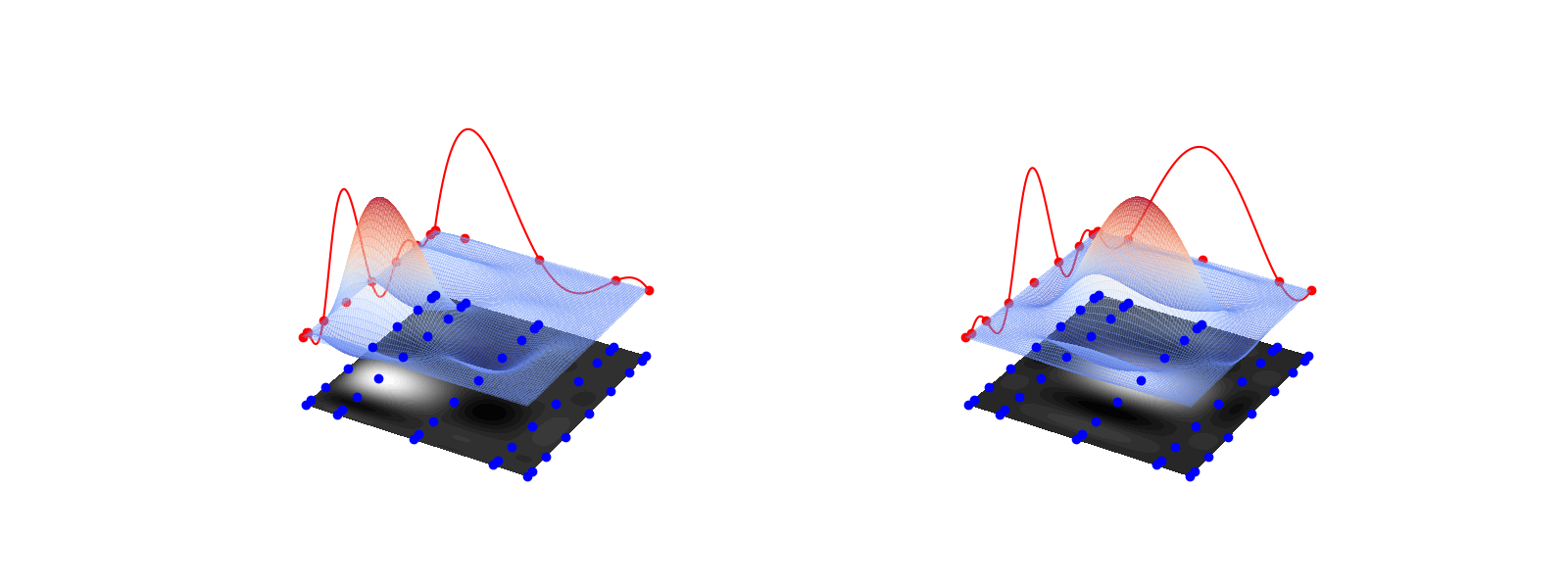
to define the univariate Lagrange polynomials. The number of points \(m(l)\) of this rule grows exponentially with the level \(l\), specifically \(m(0)=1\) and \(m(l)=2^{l}+1\) for \(l\geq1\). The univariate Clenshaw-Curtis points, the tensor-product grid \(\mathcal{Z}_{\boldsymbol{\beta}}\), and two multivariate Lagrange polynomials with their corresponding univariate Lagrange polynomials are shown below for \(\boldsymbol{\beta}=(2,2)\).

import numpy as np
from pyapprox.util.utilities import cartesian_product
from pyapprox.util.visualization import get_meshgrid_function_data, plt
from pyapprox.util.utilities import get_tensor_product_quadrature_rule
from pyapprox.surrogates.orthopoly.quadrature import clenshaw_curtis_pts_wts_1D
from pyapprox.surrogates.approximate import adaptive_approximate
from pyapprox.surrogates.interp.adaptive_sparse_grid import (
    tensor_product_refinement_indicator)
from functools import partial
from pyapprox.surrogates.orthopoly.quadrature import (
    clenshaw_curtis_in_polynomial_order, clenshaw_curtis_rule_growth)
from pyapprox.surrogates.interp.tensorprod import (
    canonical_univariate_piecewise_polynomial_quad_rule)
from pyapprox.benchmarks.benchmarks import setup_benchmark
from pyapprox.surrogates.interp.tensorprod import (
    UnivariatePiecewiseQuadraticBasis, UnivariateLagrangeBasis,
    TensorProductInterpolant, TensorProductBasis)

nnodes_1d = [5, 9]
nodes_1d = [-np.cos(np.arange(nnodes)*np.pi/(nnodes-1))
            for nnodes in nnodes_1d]
nodes = cartesian_product(nodes_1d)
lagrange_basis_1d = UnivariateLagrangeBasis()
tp_lagrange_basis = TensorProductBasis([lagrange_basis_1d]*2)

fig = plt.figure(figsize=(2*8, 6))
ax = fig.add_subplot(1, 2, 1, projection='3d')
ii, jj = 1, 3
tp_lagrange_basis.plot_single_basis(ax, nodes_1d, ii, jj, nodes)

ax = fig.add_subplot(1, 2, 2, projection='3d')
level = 2
ii, jj = 2, 4
tp_lagrange_basis.plot_single_basis(ax, nodes_1d, ii, jj, nodes)

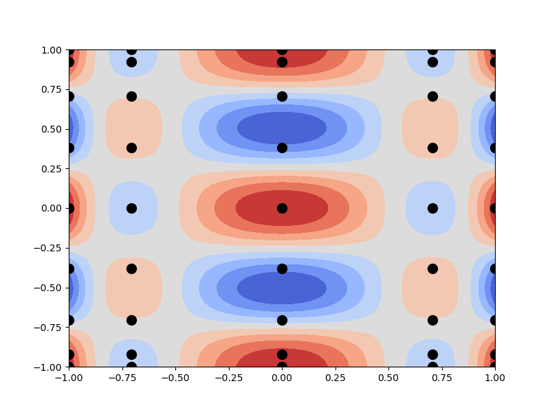
To construct a surrogate using tensor product interpolation we simply multiply all such basis functions by the value of the function \(f_\ai\) evaluated at the corresponding interpolation point. The following uses tensor product interpolation to approximate the simple function

\[f_\ai(\rv) = \cos(2\pi\rv_1)\cos(2\pi\rv_2), \qquad \rv\in\rvdom=[-1,1]^2\]

def fun(z): return (np.cos(2*np.pi*z[0, :]) *
                    np.cos(2*np.pi*z[1, :]))[:, np.newaxis]


lagrange_interpolant = TensorProductInterpolant([lagrange_basis_1d]*2)
values = fun(nodes)
lagrange_interpolant.fit(nodes_1d, values)


marker_color = 'k'
alpha = 1.0
fig, axs = plt.subplots(1, 1, figsize=(8, 6))
axs.plot(nodes[0, :], nodes[1, :], 'o',
         color=marker_color, ms=10, alpha=alpha)

plot_limits = [-1, 1, -1, 1]
num_pts_1d = 101
X, Y, Z = get_meshgrid_function_data(
    lagrange_interpolant, plot_limits, num_pts_1d)

num_contour_levels = 10
levels = np.linspace(Z.min(), Z.max(), num_contour_levels)
cset = axs.contourf(
    X, Y, Z, levels=levels, cmap="coolwarm", alpha=alpha)

The error in the tensor product interpolant is given by

\[\lVert f_\ai-f_{\ai,\bi}\rVert_{L^\infty(\rvdom)} \le C_{d,s} N_{\bi}^{-s/d}\]

where \(f_\alpha\) has continuous mixed derivatives of order \(s\).

Post-processing

Once a surrogate has been constructed it can be used for many different purposes. For example one can use it to estimate moments, perform sensitivity analysis, or simply approximate the evaluation of the expensive model at new locations where expensive simulation model data is not available.

To use the surrogate for computing moments we simply draw realizations of the input random variables \(\rv\) and evaluate the surrogate at those samples. We can approximate the mean of the expensive simluation model as the average of the surrogate values at the random samples.

We know from Monte Carlo Quadrature that the error in the Monte carlo estimate of the mean using the surrogate is

\[\begin{split}\mean{\left(Q_{\alpha}-\mean{Q}\right)^2}&=N^{-1}\var{Q_\alpha}+\left(\mean{Q_{\alpha}}-\mean{Q}\right)^2\\ &\le N^{-1}\var{Q_\alpha}+C_{d,s} N_{\bi}^{-s/d}\end{split}\]

Because a surrogate is inexpensive to evaluate the first term can be driven to zero so that only the bias remains. Thus the error in the Monte Carlo estimate of the mean using the surrogate is dominated by the error in the surrogate. If this error can be reduced more quickly than frac{N^{-1}} (as is the case for low-dimensional tensor-product interpolation) then using surrogates for computing moments is very effective.

Note that moments can be estimated without using Monte-Carlo sampling by levaraging properties of the univariate interpolation rules used to build the multi-variate interpolant. Specifically, the expectation of a tensor product interpolant can be computed without explicitly forming the interpolant and is given by

\[\mu_{\bi}=\int_{\rvdom} \sum_{\V{j}\le\bi}f_\ai(\rv^{(\V{j})})\prod_{i=1}^d\phi_{i,j_i}(\rv_i) w(\rv)\,d\rv=\sum_{\V{j}\le\bi} f_\ai(\rv^{(\V{j})}) v_{\V{j}}.\]

The expectation is simply the weighted sum of the Cartesian-product of the univariate quadrature weights

\[v_{\V{j}}=\prod_{i=1}^d\int_{\rvdom_i}{\phi_{i,j_i}(\rv_i)}\,dw(\rv_i),\]

which can be computed analytically.

x, w = get_tensor_product_quadrature_rule(level, 2, clenshaw_curtis_pts_wts_1D)
surrogate_mean = fun(x)[:, 0].dot(w)
print('Quadrature mean', surrogate_mean)

Quadrature mean 0.10540659444426355

Here we have recomptued the values of \(f\) at the interpolation samples, but in practice we sould just re-use the values collected when building the interpolant.

Now let us compare the quadrature mean with the MC mean computed using the surrogate

num_samples = int(1e6)
samples = np.random.uniform(-1, 1, (2, num_samples))
values = lagrange_interpolant(samples)
mc_mean = values.mean()
print('Monte Carlo surrogate mean', mc_mean)

Monte Carlo surrogate mean -0.00010377793672674781

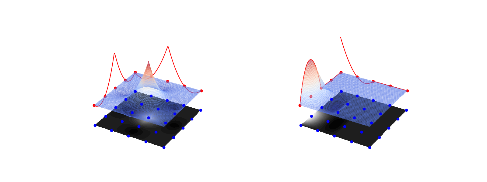
Piecewise-polynomial approximation

Polynomial interpolation accurately approximates smooth functions, however its accuracy degrades as the regularity of the target function decreases. For piecewise continuous functions, or functions with only a limited number of continuous derivaties, piecewise-polynomial approximation may be more appropriate.

The following plots two piecewise-quadratic basis functions in 2D

fig = plt.figure(figsize=(2*8, 6))
nnodes_1d = [5, 5]
nodes_1d = [np.linspace(-1, 1, nnodes) for nnodes in nnodes_1d]
nodes = cartesian_product(nodes_1d)
tp_quadratic_basis = TensorProductBasis(
    [UnivariatePiecewiseQuadraticBasis()]*2)
ax = fig.add_subplot(1, 2, 1, projection='3d')
tp_quadratic_basis.plot_single_basis(ax, nodes_1d, 2, 2, nodes)
ax = fig.add_subplot(1, 2, 2, projection='3d')
tp_quadratic_basis.plot_single_basis(ax, nodes_1d, 0, 1, nodes)

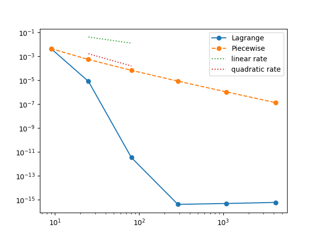
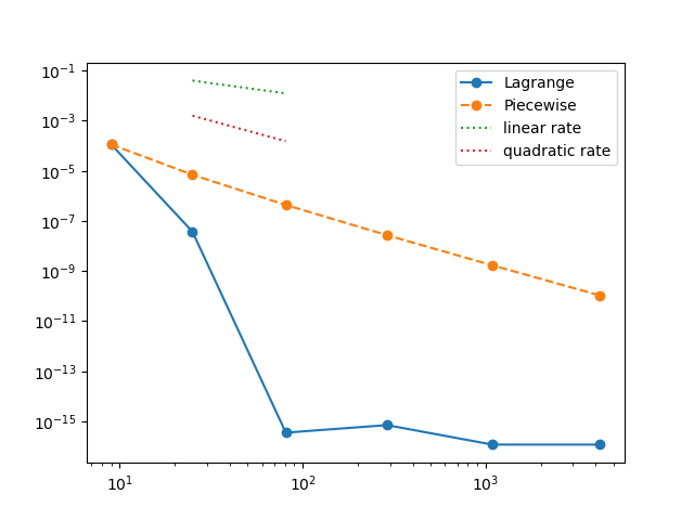
The following compares the convergence of Lagrange and picewise polynomial tensor product interpolants. Change the benchmark to see the effect of smoothness on the approximation accuracy.

First define wrappers to build the tensor product interpolants

def build_lagrange_tp(max_level_1d):
    univariate_quad_rule_info = [
        clenshaw_curtis_in_polynomial_order, clenshaw_curtis_rule_growth,
        None, None]
    return adaptive_approximate(
        benchmark.fun, benchmark.variable, "sparse_grid",
        {"refinement_indicator": tensor_product_refinement_indicator,
         "max_level_1d": max_level_1d,
         "univariate_quad_rule_info": univariate_quad_rule_info,
         "max_nsamples": np.inf}).approx


def build_piecewise_tp(max_level_1d):
    basis_type = "quadratic"
    # basis_type = "linear"
    univariate_quad_rule_info = [
        partial(canonical_univariate_piecewise_polynomial_quad_rule,
                basis_type),
        clenshaw_curtis_rule_growth, None, None]
    return adaptive_approximate(
        benchmark.fun, benchmark.variable, "sparse_grid",
        {"refinement_indicator": tensor_product_refinement_indicator,
         "max_level_1d": max_level_1d,
         "univariate_quad_rule_info": univariate_quad_rule_info,
         "basis_type": basis_type, "max_nsamples": np.inf}).approx

Load a benchmark

nvars = 2
benchmark = setup_benchmark("genz", nvars=nvars, test_name="oscillatory")
# benchmark = setup_benchmark("genz", nvars=nvars, test_name="c0continuous",
#                            c_factor=0.5, w=0.5)

Run a convergence study

validation_samples = benchmark.variable.rvs(1000)
validation_values = benchmark.fun(validation_samples)

piecewise_data = []
lagrange_data = []
for level in range(1, 7):   # nvars = 2
# for level in range(1, 4):  # nvars = 3
    ltp = build_lagrange_tp(level)
    lvalues = ltp(validation_samples)
    lerror = np.linalg.norm(validation_values-lvalues)/np.linalg.norm(
        validation_values)
    lagrange_data.append([ltp.samples.shape[1], lerror])
    ptp = build_piecewise_tp(level)
    pvalues = ptp(validation_samples)
    perror = np.linalg.norm(validation_values-pvalues)/np.linalg.norm(
        validation_values)
    piecewise_data.append([ptp.samples.shape[1], perror])
lagrange_data = np.array(lagrange_data).T
piecewise_data = np.array(piecewise_data).T

ax = plt.subplots()[1]
ax.loglog(*lagrange_data, '-o', label='Lagrange')
ax.loglog(*piecewise_data, '--o', label='Piecewise')
work = piecewise_data[0][1:3]
ax.loglog(work, work**(-1.0), ':', label='linear rate')
ax.loglog(work, work**(-2.0), ':', label='quadratic rate')
_ = ax.legend()

Similar behavior occurs when using quadrature.

Load in the benchmark.

nvars = 2
benchmark = setup_benchmark("genz", nvars=nvars, test_name="oscillatory")

Run a convergence study

piecewise_data = []
lagrange_data = []
for level in range(1, 7):   # nvars = 2
    ltp = build_lagrange_tp(level)
    lvalues = ltp.moments()[0, 0]
    lerror = np.linalg.norm(benchmark.mean-lvalues)/np.linalg.norm(
        benchmark.mean)
    lagrange_data.append([ltp.samples.shape[1], lerror])
    ptp = build_piecewise_tp(level)
    pvalues = ptp.moments()[0, 0]
    perror = np.linalg.norm(benchmark.mean-pvalues)/np.linalg.norm(
        benchmark.mean)
    piecewise_data.append([ptp.samples.shape[1], perror])
lagrange_data = np.array(lagrange_data).T
piecewise_data = np.array(piecewise_data).T

ax = plt.subplots()[1]
ax.loglog(*lagrange_data, '-o', label='Lagrange')
ax.loglog(*piecewise_data, '--o', label='Piecewise')
work = piecewise_data[0][1:3]
ax.loglog(work, work**(-1.0), ':', label='linear rate')
ax.loglog(work, work**(-2.0), ':', label='quadratic rate')
_ = ax.legend()

References

[XKSISC2002]

D. Xiu and G.E. Karniadakis. The Wiener-Askey Polynomial Chaos for stochastic differential equations. SIAM J. Sci. Comput., 24(2), 619-644, 2002.

[RWMIT2006]

C.E Rasmussen and C. Williams. Gaussian Processes for Machine Learning. MIT Press, 2006.

[BGAN2004]

H. Bungartz and M. Griebel. Sparse Grids. Acta Numerica, 13, 147-269, 2004.

[SFIJNME2017]

C Soize and C. Farhat. A nonparametric probabilistic approach for quantifying uncertainties in low-dimensional and high-dimensional nonlinear models. International Journal for Numerical Methods in Engineering, 109(6), 837-888, 2017.