Monte Carlo Quadrature: Beyond Mean Estimation

Monte Carlo Quadrature discussed how to use Monte Carlo quadrature to compute the mean of a model. In contrast, this tutorial shows how to use MC to compute alternative statistics of a model, for example variance, and how to compute the MSE of MC estimates of such statistics.

In this tutorial we will discuss using MC to estimate the mean \(\mat{\mu}\) and covariance \(\mat{\Sigma}\) of a vector-valued function \(f_\alpha:\reals^D\to\reals^K\), with entries respectively given by

\[(\mat{Q}_{\alpha}^\mu)_k=\int_\rvdom f_{\alpha,k}(\rv)\pdf(\rv)\dx{\rv} \qquad k=1,\ldots,K\]

\[(\mat{Q}_{\alpha}^{\Sigma})_{jk}=\int_\rvdom \left(f_{\alpha,j}^2(\rv)-Q_{\alpha,j}^\mu\right)\left(f_{\alpha,k}(\rv)-Q_{\alpha,k}^\mu\right)^\top\pdf(\rv)\dx{\rv}, \qquad j,k=1,\ldots,K.\]

Moreover, we will show how to estimate a vector-valued statistics that may be comprised of multiple statistics of a scalar function, a single statistics of a vector-valued function, or a combination of both.

In the most general case, the vector valued statistic comprised of \(S\) different statistics

\[\mat{Q}_\alpha=[(Q_{\alpha})_1,\ldots,(Q_{\alpha})_S]^\top \in \reals^{S},\]

As an example, in the following we will show how to use MC to compute the mean and covariance \(\mat{\Sigma}\) of a vector-valued function \(f_\alpha:\reals^D\to\reals^K\), that is

\[\mat{Q}_\alpha=[(\mat{Q}_{\alpha}^\mu)^\top, \text{flat}(\mat{Q}_{\alpha}^{\Sigma})^\top]^\top\in\reals^{K+K^2}.\]

where for a general matrix \(\mat{X}\in\reals^{M\times N}\)

\[\text{flat}(\mat{X})=[X_{11}, \ldots, X_{1N}, \ldots, X_{M1}, \ldots, X_{MN}]^\top \in \reals^{MN}.\]

Specifically, we will consider

\[f_0(\rv) = [\sqrt{11}\rv^5, \rv^4, \sin(2\pi \rv)]^\top\]

To compute a vector-valued statistic we follow the same procedure introduced for estimating the mean of a scalar function but now compute MC estimators for each statistic and function, that is

\[(Q^\mu_{\alpha}(\rvset_N))_k= N^{-1}\sum_{n=1}^N f_{\alpha, k}^{(n)}, \qquad k=1,\ldots, K\]

\[(Q^{\Sigma}_{\alpha}(\rvset_N))_{jk}= (N-1)^{-1}\sum_{n=1}^N \left( f_{\alpha, j}^{(n)}-(Q^\mu_{\alpha}(\rvset_N))_j\right)\left( f_{\alpha, k}^{(n)}-(Q^\mu_{\alpha}(\rvset_N))_k\right), \quad j,k=1,\ldots, K.\]

The following implements this procedure.

First load the benchmark

import numpy as np
import matplotlib.pyplot as plt

from pyapprox.benchmarks import setup_benchmark
from pyapprox.multifidelity.factory import get_estimator, multioutput_stats

np.random.seed(1)
benchmark = setup_benchmark("multioutput_model_ensemble")

Now construct the estimator. The following requires the costs of the model the covariance and some other quantities W and B. These four quantities are not needed to compute the value of the estimator from a sample set, however they are needed to compute the MSE of the estimator and the number of samples of that model for a given target cost. We load these quantities but ignore there meaning for the moment.

costs = np.array([1])
nqoi = 3
cov = benchmark.covariance[:3, :3]
W = benchmark.fun.covariance_of_centered_values_kronker_product()[:9, :9]
B = benchmark.fun.covariance_of_mean_and_variance_estimators()[:3, :9]

target_cost = 10
stat = multioutput_stats["mean_variance"](nqoi)
stat.set_pilot_quantities(cov, W, B)
est = get_estimator("mc", stat, costs)
est.allocate_samples(target_cost)
samples = est.generate_samples_per_model(benchmark.variable.rvs)[0]
values = benchmark.funs[0](samples)
stats = est(values)

The following compares the estimated value with the true values. We are only extracting certain components from the benchmark because the benchmark is designed for estimating vector-valued statistics with multiple models, but we are ignoring the other models for now.

print(benchmark.mean[0])
print(stats[:3])
print(benchmark.covariance[:3, :3])
print(stats[3:].reshape(3, 3))

[ 5.52770798e-01  2.00000000e-01 -7.60350892e-17]
[0.08939676 0.04328916 0.3916164 ]
[[ 0.69444444  0.22110832 -0.30108393]
 [ 0.22110832  0.07111111 -0.11077764]
 [-0.30108393 -0.11077764  0.5       ]]
[[ 0.03995681  0.01661502 -0.10618668]
 [ 0.01661502  0.00696109 -0.04480152]
 [-0.10618668 -0.04480152  0.38481283]]

Similarly to a MC estimator for a scalar, a vector-valued MC estimator is a random variable. Assuming that we are not using an approximation of the model we care about, the error in the MC estimator is characterized completely by the covariance of the estimator statistics. The following draws from [DWBG2024] and shows how to compute the estimator covariance. We present general formula for the covariance between estimators of using different vector-valued models \(f_\alpha\text{ and }f_\beta\) and using sample sets \(\rvset_N, \rvset_M\) of (potentially) different sizes.

Mean Estimation

First consider the estimation of the mean. The covariance between two estimates of the mean that share P samples, i.e. \(P=|\rvset_\alpha\cup \rvset_\beta|\), is

\[\covar{\mat{Q}^\mu_\alpha(\rvset_{N})}{\mat{Q}^\mu_\beta(\rvset_{M})} = \frac{P}{MN}\covar{f_\alpha}{f_\beta} \quad \in\reals^{K\times K}\]

Variance Estimation

The covariance between two estimators of variance is

\[\covar{\mat{Q}_\alpha^{\Sigma}(\rvset_{N})}{\mat{Q}_\beta^{\Sigma}(\rvset_{M})} = \frac{P(P-1)}{M(M-1)N(N-1)}\mat{V}_{\alpha,\beta}+\frac{P}{MN}\mat{W}_{\alpha,\beta} \quad \in\reals^{K^2\times K^2}\]

where

\[\mat{V}_{\alpha,\beta} = \covar{f_\alpha}{f_\beta}^{\otimes2}+(\mat{1}_K^\top\otimes\covar{f_\alpha}{f_\beta}\otimes\mat{1}_K)\circ(\mat{1}_K\otimes\covar{f_\alpha}{f_\beta}\otimes\mat{1}_K^\top),\quad \in \reals^{K^2\times K^2}\]

\[\mat{W}_{\alpha,\beta} = \covar{(f_\alpha-\mean{f_\alpha})^{\otimes 2}}{(f_\beta-\mean{f_\beta})^{\otimes 2}} \quad \in \reals^{K^2\times K^2}\]

Above we used the notation, for general matrices \(\mat{X},\mat{Y}\),

\[\mat{X}\otimes \mat{Y}=\text{flat}(\mat{X}\mat{Y}^\top)\]

for a flattened outer product,

\[\mat{X}\circ \mat{Y}\]

for an element wise product, and

\[X^{\otimes2}=\mat{X}\otimes \mat{X}\]

Simultaneous Mean and Variance Estimation

The covariance between two estimators of mean and variance of the form

\[\mat{Q}_\alpha^{\mu,\Sigma}(\rvset_{N})=[\mat{Q}_\alpha^{\mu}(\rvset_{N}), \mat{Q}_\alpha^{\Sigma}(\rvset_{N})]^\top \quad \in\reals^{(K+K^2)\times (K+K^2)}\]

is

\[\begin{split}\covar{\mat{Q}_\alpha^{\mu,\Sigma}(\rvset_{N})}{\mat{Q}_\beta^{\mu,\Sigma}(\rvset_{M})} = \begin{bmatrix}\covar{\mat{Q}_\alpha^\mu(\rvset_{N})}{\mat{Q}_\beta^\mu(\rvset_{N})} & \covar{\mat{Q}_\alpha^\mu(\rvset_{N})}{\mat{Q}_\beta^{\Sigma}(\rvset_{M})}\\ \covar{\mat{Q}_\alpha^{\Sigma}(\rvset_{M})}{\mat{Q}_\beta^\mu(\rvset_{N})}& \covar{\mat{Q}_\alpha^{\Sigma}(\rvset_{M})}{\mat{Q}_\beta^{\Sigma}(\rvset_{M})}\end{bmatrix}\end{split}\]

We have already shown the form of the upper and lower diagonal blocks. The off diagonal blocks are

\[\covar{\mat{Q}_\alpha^\mu(\rvset_{N})}{\mat{Q}_\beta^{\Sigma}(\rvset_{M})}=\frac{P}{MN}\mat{B}_{\alpha,\beta}\quad\in\reals^{K\times K^2}\]

where

\[\mat{B}_{\alpha,\beta}=\covar{f_\alpha}{(f_\beta-\mean{f_\beta})^{\otimes 2}}\quad\in\reals^{K\times K^2}\]

MSE

For vector valued statistics, the MSE formular presented in the previous tutorial no longer makes sense because the estimator is a multivariate random variable with a mean and covariance (not a mean and variance like for the scalar formulation). Consequently, for an unbiased estimator, the error in a vector-valued statistic is usually a scalar function of the estimator covariance. Two common choices are the determinant and trace of the estimator covariance.

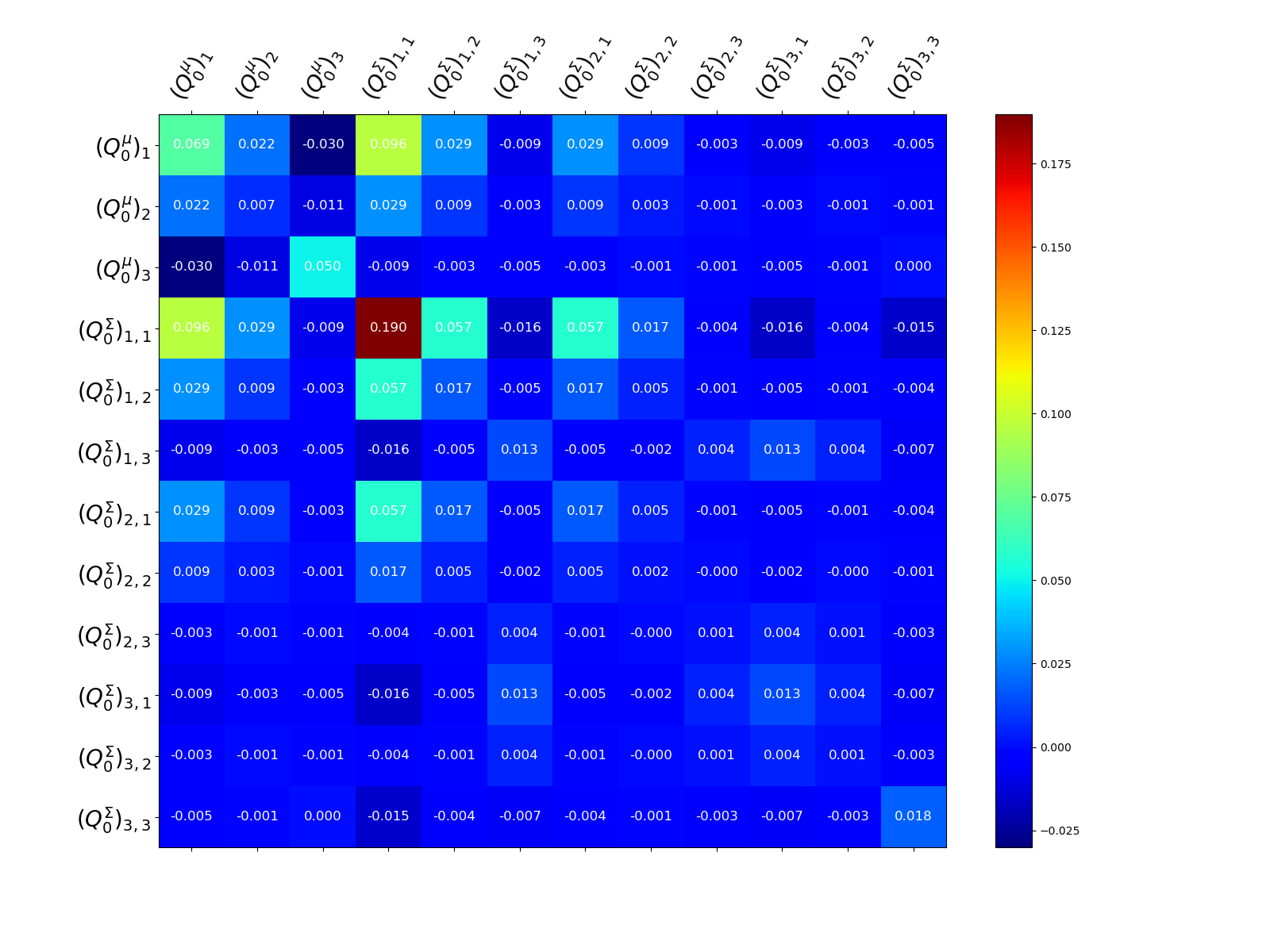
The estimator covariance can be obtained using

from pyapprox.multifidelity.visualize import plot_correlation_matrix
# plot correlation matrix can also be used for covariance matrics
labels = ([r"$(Q^{\mu}_{0})_{%d}$" % (ii+1) for ii in range(nqoi)] +
          [r"$(Q^{\Sigma}_{0})_{%d,%d}$" % (ii+1, jj+1)
           for ii in range(nqoi) for jj in range(nqoi)])
ax = plt.subplots(1, 1, figsize=(2*8, 2*6))[1]
_ = plot_correlation_matrix(
    est.optimized_covariance(), ax=ax, model_names=labels, label_fontsize=20)

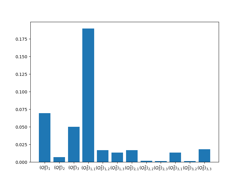
We can plot the diagonal, which contains the estimator variances that would be obtained if each statistic was treated individually.

ax = plt.subplots(1, 1, figsize=(8, 6))[1]
est_variances = np.diag(est.optimized_covariance().numpy())
_ = plt.bar(labels, est_variances)

Remarks

Similar experssions to those above for scalar outputs can be found in [QPOVW2018].

Video

Click on the image below to view a video tutorial on multi-output Monte Carlo quadrature

References

[DWBG2024]

T. Dixon et al. Covariance Expressions for Multi-Fidelity Sampling with Multi-Output, Multi-Statistic Estimators: Application to Approximate Control Variates. 2024

[QPOVW2018]

Multifidelity Monte Carlo Estimation of Variance and Sensitivity Indices E. Qian, B. Peherstorfer, D. OMalley, V. V. Vesselinov, and K. Willcox. SIAM/ASA Journal on Uncertainty Quantification 2018 6:2, 683-706