Approximate Control Variate Allocation Matrices

Optimizing and constructing PACV estimators requires estimating $\mathbb{C}\text{ov}[Q_0,\mathrm{\Delta }]$ and $\mathbb{C}\text{ov}[\mathrm{\Delta },\mathrm{\Delta }]$ which depend on the statistical properties of the models being used but also on the sample alloaction how independent sample sets are shared among the sample sets ${\mathcal{Z}}_{\alpha }\text{ and }{\mathcal{Z}}_{\alpha }^{\ast }$.

For example, when computing the mean of a scalar model when the covariance between models is given by $\mathbf{C}$ and the first row of $\mathbf{C}$ is $\mathbf{c}$ then

$$\mathbb{C}\text{ov}[Q_0,\mathbf{\Delta }]=\mathbf{g}\circ \mathbf{c}$$

$$g_i=\frac{N_{i^{\ast }\cap 0}}{N_{i^{\ast }}{N}_0}-\frac{N_{i\cap 0}}{N_i{N}_0},i=1,\dots ,M$$

and

$$\mathbb{C}\text{ov}[\mathbf{\Delta },\mathbf{\Delta }]=\mathbf{G}\circ \mathbf{C}$$

$$G_{ij}=\frac{N_{i^{\ast }\cap j^{\ast }}}{N_{i^{\ast }}{N}_{j^{\ast }}}-\frac{N_{i^{\ast }\cap j}}{N_{i^{\ast }}{N}_j}-\frac{N_{i\cap j^{\ast }}}{N_i{N}_{j^{\ast }}}+\frac{N_{i\cap j}}{N_i{N}_j},i,j=1,\dots ,M$$

where $\circ$ is the Haddamard (element-wise) product.

The implementation of PACV uses allocation matrices $\mathbf{A}$ that encode how independent sample sets are shared among the sample sets ${\mathcal{Z}}_{\alpha }\text{ and }{\mathcal{Z}}_{\alpha }^{\ast }$.

For example, the allocation matrix of ACVMF using $M=3$ low-fidelity models (GMF with recursion index $(0,0,0)$) is

$$\begin{array}{r}\mathbf{A}=\left[\begin{array}{cccccccc}0& 1& 1& 1& 1& 1& 1& 1\\ 0& 0& 0& 1& 0& 1& 0& 1\\ 0& 0& 0& 0& 0& 1& 0& 1\\ 0& 0& 0& 0& 0& 0& 0& 1\end{array}\right]\end{array}$$

An entry of one indicates in the ith row of the jth column indicates that the ith independent sample set is used in the corresponding set ${\mathcal{Z}}_j$ if j is odd or ${\mathcal{Z}}_j^{\ast }$ if j is even. The first column will always only contain zeros because the set ${\mathcal{Z}}_0^{\ast }$ is never used by ACV estimators.

Note, here we focus on how to construct and use allocation matrices for ACVMF like PACV estimtors. However, much of the discussion carries over to other estimators like those based on recursive difference and ACVIS.

The allocation matrix together with the number of points $\mathbf{p}=[p_0,\dots ,p_M{]}^{\mathrm{\top }}$ in the each independent sample set which we call partitions can be used to determine the number of points in the intersection of the sets ${\mathcal{Z}}_{\alpha }\text{ and }{\mathcal{Z}}_{\beta }$, where $\alpha \text{ and }\beta$ may be unstarred or starred. Intersection matrices are used to compute $\mathbb{C}\text{ov}[Q_0,\mathrm{\Delta }]$ and $\mathbb{C}\text{ov}[\mathrm{\Delta },\mathrm{\Delta }]$. The number of intersection points can be represented by a $2(M+1)\times 2(M+1)$ matrix

$$\begin{array}{r}\mathbf{B}=\left[\begin{array}{cccccccc}0& 0& 0& 0& 0& 0& 0& 0\\ 0& N_{0\cup 0}& N_{0\cup 1}& N_{0\cup 1^{\ast }}& N_{0\cup 2}& N_{0\cup 2^{\ast }}& N_{0\cup 3}& N_{0\cup 3^{\ast }}\\ 0& N_{1^{\ast }\cup 0}& N_{1^{\ast }\cup 1^{\ast }}& N_{1^{\ast }\cup 1}& N_{1^{\ast }\cup 2^{\ast }}& N_{1^{\ast }\cup 2}& N_{1^{\ast }\cup 3^{\ast }}& N_{1^{\ast }\cup 3}\\ 0& N_{1\cup 0}& N_{1\cup 1^{\ast }}& N_{1\cup 1}& N_{1\cup 2^{\ast }}& N_{1\cup 2}& N_{1\cup 3^{\ast }}& N_{1\cup 3}\\ ⋮& ⋮& ⋮& ⋮& ⋮& ⋮& ⋮& ⋮\\ 0& N_{3^{\star }\cup 0}& N_{3^{\star }\cup 1^{\ast }}& N_{3^{\star }\cup 1}& N_{3^{\star }\cup 2^{\ast }}& N_{3^{\star }\cup 2}& N_{3^{\star }\cup 3^{\ast }}& N_{3^{\star }\cup 3}\\ 0& N_{3\cup 0}& N_{3\cup 1^{\ast }}& N_{3\cup 1}& N_{3\cup 2^{\ast }}& N_{3\cup 2}& N_{3\cup 3^{\ast }}& N_{3\cup 3}\end{array}\right]\end{array}$$

Defining

$$\mathbf{S}=\text{Diag}(\mathbf{p})\mathbf{A},$$

each entry of B can be computed using

$$B_{ij}=\sum _{k=0}^{2M+1}{S}_{kj}\chi [A_{ki}]$$

where

$$\begin{array}{r}\chi [A_{ki}]=\{\begin{array}{ll}1& A_{ki}=1\\ 0& A_{ki}=0\end{array}\end{array}$$

Note computing $\mathbb{C}\text{ov}[Q_0,\mathrm{\Delta }]$ and $\mathbb{C}\text{ov}[\mathrm{\Delta },\mathrm{\Delta }]$ also requires the number of samples $N_{\alpha }$, $N_{{\alpha }^{\ast }}$ in each ACV sample set ${\mathcal{Z}}_{\alpha },{\mathcal{Z}}_{\alpha }^{\ast }$ which can be computed by simply summing the rows of S or more simply extracting the relevant entry from the diagonal of B. For example

$$N_3=N_{3\cap 3}\text{ and }{N}_{3^{\ast }}=N_{3^{\ast }\cap 3^{\ast }}$$

Finally, to compute the computational cost of the estimator we must be able to compute the number of samples per model. The number of samples of the ith

$$\sum _{k=1}^M{p}_k\chi [A_{2i,k}+A_{2i+1,k}]$$

where $\chi [A_{2i,k}+A_{2i+1,k}]=1$ if $A_{2i,k}+A_{2i+1,k}>0$ and is zero otherwise.

Using our example, the intersection matrix is

$$\mathbf{p}=[2,3,4,5]$$

$$\begin{array}{r}\mathbf{S}=\left[\begin{array}{cccccccc}0& 2& 2& 2& 2& 2& 2& 2\\ 0& 0& 0& 3& 0& 3& 0& 3\\ 0& 0& 0& 0& 0& 4& 0& 4\\ 0& 0& 0& 0& 0& 5& 0& 0\end{array}\right]\end{array}$$

So summing each column of S we have

$$N_0^{\ast }=0,N_0=2,N_1^{\ast }=2,N_1=5,N_2^{\ast }=2,N_2=14,N_3^{\ast }=2,N_3=9,$$

And

$$\begin{array}{r}\mathbf{B}=\left[\begin{array}{cccccccc}0& 0& 0& 0& 0& 0& 0& 0\\ 0& 2& 2& 2& 2& 2& 2& 2\\ 0& 2& 2& 2& 2& 2& 2& 2\\ 0& 2& 2& 5& 2& 5& 2& 5\\ 0& 2& 2& 2& 2& 2& 2& 2\\ 0& 2& 2& 5& 2& 14& 2& 9\\ 0& 2& 2& 2& 2& 2& 2& 2\\ 0& 2& 2& 5& 2& 9& 2& 9\end{array}\right]\end{array}$$

The first row and column are all zero because ${\mathcal{Z}}_0^{\ast }$ is always empty.

As an example the thrid entry from the right on the bottom row corresponds to $B_{75}=N_{3\cup 2}$ which is computed by finding the rows in R that have non zero entries which are the first three rows. Then the $B_{75}$ is the sum of these rows in the 5 column of S, i.e. $2+3+4=9$.

Examples of different allocation matrices

The following lists some example alloaction matrices for the parameterically defined ACV estimators based on the general structure of ACVMF.

MFMC $(0,1,2)$

$$\begin{array}{r}\left[\begin{array}{cccccccc}0& 1& 1& 1& 1& 1& 1& 1\\ 0& 0& 0& 1& 1& 1& 1& 1\\ 0& 0& 0& 0& 0& 1& 1& 1\\ 0& 0& 0& 0& 0& 0& 0& 1\end{array}\right]\end{array}$$

$(0,0,1)$

$$\begin{array}{r}\left[\begin{array}{cccccccc}0& 1& 1& 1& 1& 1& 1& 1\\ 0& 0& 0& 1& 0& 1& 1& 1\\ 0& 0& 0& 0& 0& 1& 0& 1\\ 0& 0& 0& 0& 0& 0& 0& 1\end{array}\right]\end{array}$$

$(0,0,2)$

$$\begin{array}{r}\left[\begin{array}{cccccccc}0& 1& 1& 1& 1& 1& 1& 1\\ 0& 0& 0& 1& 0& 1& 1& 1\\ 0& 0& 0& 0& 0& 1& 1& 1\\ 0& 0& 0& 0& 0& 0& 0& 1\end{array}\right]\end{array}$$

$(0,1,1)$

$$\begin{array}{r}\left[\begin{array}{cccccccc}0& 1& 1& 1& 1& 1& 1& 1\\ 0& 0& 0& 1& 1& 1& 1& 1\\ 0& 0& 0& 0& 0& 1& 0& 1\\ 0& 0& 0& 0& 0& 0& 0& 1\end{array}\right]\end{array}$$

How to construct ACVMF like allocation matrices

The following shows the general procedure to construct ACVMF like estimators for a recursion index

$$\gamma =({\gamma }_1,\dots ,{\gamma }_M)$$

As a concrete example, consider the recursion index $\gamma =(0,0,1)$.

First we set $A_{2\alpha +1,\alpha }=1$ for all $\alpha =0,\dots ,M$

E.g. for (0,0,1)

$$\begin{array}{r}\left[\begin{array}{cccccccc}0& 1& 0& 0& 0& 0& 0& 0\\ 0& 0& 0& 1& 0& 0& 0& 0\\ 0& 0& 0& 0& 0& 1& 0& 0\\ 0& 0& 0& 0& 0& 0& 0& 1\end{array}\right]\end{array}$$

We then set $A_{2\alpha ,{\gamma }_{\alpha }}=1$ for $\alpha =1,\dots ,M$. For example,

$$\begin{array}{r}\left[\begin{array}{cccccccc}0& 1& 1& 0& 1& 0& 0& 0\\ 0& 0& 0& 1& 0& 0& 1& 0\\ 0& 0& 0& 0& 0& 1& 0& 0\\ 0& 0& 0& 0& 0& 0& 0& 1\end{array}\right]\end{array}$$

And finally because ACMF always uses all independent partitions up to including ${\gamma }_{\alpha }$ we set $A_{i,k}=1$, for $k=0,\dots ,{\gamma }_{\alpha }$ and $\mathrm{\forall }i$. For example

$$\begin{array}{r}\left[\begin{array}{cccccccc}0& 1& 1& 1& 1& 1& 1& 1\\ 0& 0& 0& 1& 0& 1& 1& 1\\ 0& 0& 0& 0& 0& 1& 0& 1\\ 0& 0& 0& 0& 0& 0& 0& 1\end{array}\right]\end{array}$$

The following can be used to plot the allocation matrix of any PACV estimator (not just GMF). Note we load a benchmark because it is needed to initialize the PACV estimator, but the allocation matrix is independent of any benchmark properties other than the number of models it provides

import matplotlib.pyplot as plt

from pyapprox.benchmarks import setup_benchmark
from pyapprox.multifidelity.factory import get_estimator, multioutput_stats

benchmark = setup_benchmark("tunable_model_ensemble")
model = benchmark.fun

stat = multioutput_stats["mean"](benchmark.nqoi)
stat.set_pilot_quantities(benchmark.covariance)
est = get_estimator("grd", stat, model.costs(), recursion_index=(2, 0))

ax = plt.subplots(1, 1, figsize=(8, 6))[1]
_ = est.plot_allocation(ax)

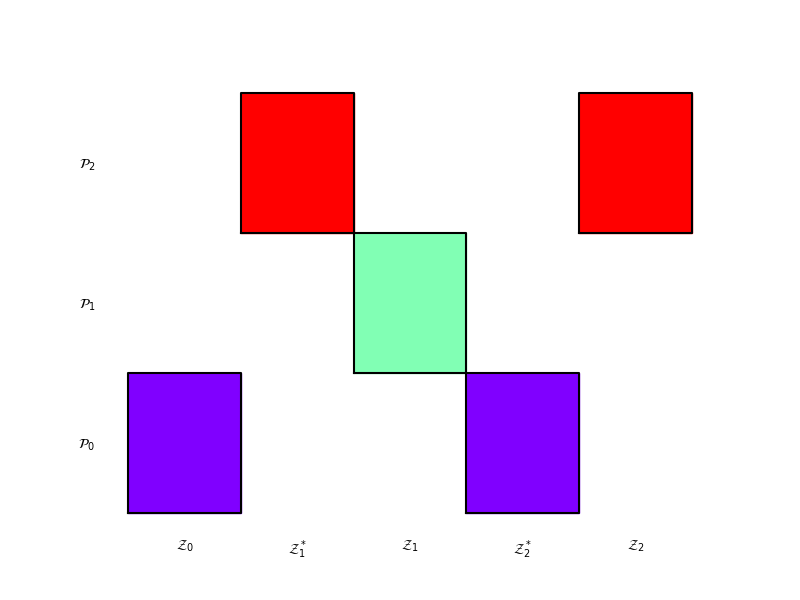
The different colors represent different independent sample partitions. Subsets ${\mathcal{Z}}_{\alpha }\text{ or }{\mathcal{Z}}_{\alpha }^{\ast }$ having the same color, means that the same set of samples are used in each subset.

Try changing recursion index to (0, 1) or (2, 0) and the estimator from “gis” to “gmf” or” grd”

Evaluating a PACV estimator

Allocation matrices are also useful for evaluating a PACV estimator. To evaluate the ACV estimator we must construct each independent sample partition from a set of $N_{\text{tot}}$ samples ${\mathcal{Z}}_{\text{tot}}$ where

$$N_{\text{tot}}=\sum _{\alpha =0}^M{p}_{\alpha }$$

We then must allocate each model on a subset of these samples dictated by the allocation matrix. For a model index $\alpha$ we must evaluate a model at a independent partition k if $A_{2\alpha ,k}=1$ or $A_{2\alpha +1,k}=1$. These correspond to the sets ${\mathcal{Z}}_{\alpha }^{\ast },{\mathcal{Z}}_{\alpha }$. We store these active partitions in a flattened sample array for each model ordered by increasing partition index, which is passed to each user. E.g. if the partitions 0, 1, 3 are active then we store $[{\mathcal{Z}}_0^{†},{\mathcal{Z}}_1^{†},{\mathcal{Z}}_3^{†}]$ where the dagger indicates the samples sets are associated with partitions and not the estimator sets ${\mathcal{Z}}_{{\alpha }^{\ast }},{\mathcal{Z}}_{\alpha }$.

The user can then evaluate each model without knowing anything about the ACV estimator sets or the independent partitions.

These model evaluations are then passed back to the estimator and internally we must assigne the values to each ACV estimator sample set. Specifically for each model $\alpha$, we loop through all partition indices k and if $A_{2\alpha ,k}=1$ we assign ${\mathcal{f}}_{\alpha }\mathcal{(}{\mathcal{Z}}_{\mathcal{k}}^{†}\mathcal{)}$ to ${\mathcal{Z}}_{{\alpha }^{\ast }}$ similarly if $A_{2\alpha +1,k}=1$ we assign ${\mathcal{f}}_{\alpha }\mathcal{(}{\mathcal{Z}}_{\mathcal{k}}^{†}\mathcal{)}$ to ${\mathcal{Z}}_{\alpha }$.