Convergence studies

This tutorial demonstrates how to investigate the convergence of parameterized numerical approximations, for example tensor product quadrature or numerical models used to solve partial differential equations with unknown inputs.

First lets define a Integrator class which can be used to integrate multivariate functions with tensor product quadrature, that is compute

\[I(\rv) = \int_D f(x, \rv)dx\]

from scipy import stats
import numpy as np

from pyapprox.analysis.convergence_studies import (
    run_convergence_study, plot_convergence_data)
from pyapprox.surrogates import (
    get_tensor_product_piecewise_polynomial_quadrature_rule)
from pyapprox.interface import (
    evaluate_1darray_function_on_2d_array, WorkTrackingModel,
    TimerModel)
from pyapprox.variables import (
    IndependentMarginalsVariable, ConfigureVariableTransformation)


class Integrator(object):
    def __init__(self, integrand):
        self.integrand = integrand

    def set_quad_rule(self, nsamples_1d):
        self.xquad, self.wquad = \
            get_tensor_product_piecewise_polynomial_quadrature_rule(
                nsamples_1d, [0, 1, 0, 1], degree=1)

    def integrate(self, sample):
        self.set_quad_rule(sample[-2:].astype(int))
        val = self.integrand(sample[:-2], self.xquad)[:, 0].dot(self.wquad)
        return val

    def __call__(self, samples):
        return evaluate_1darray_function_on_2d_array(
            self.integrate, samples, None)

    @staticmethod
    def get_num_degrees_of_freedom(config_sample):
        return np.prod(config_sample)

To assess convergence we will use the function run_convergence_study. This routine requires a function that takes samples that consist of realizations of the random variables concatenated with any configuration variables which define the numerical resolution of the quadrature rule, in this case the number of quadrature points used in the first and second dimension.

To demonstrate its usage lets integrate the function

\[f(x, \rv)=\rv_1(x_1^2+x_2^2)\]

were \(z\) is a uniform variable on \([0, 1]\). Now define this integrand and the true value as a function of the random samples.

variable = IndependentMarginalsVariable([stats.uniform(0, 1)])


def integrand(sample, x):
    return np.sum(sample[0]*x**2, axis=0)[:, None]


def true_value(samples):
    return 2/3*samples.T

We must also define the permissible values of the configuration variables that define the number of points \(n_1, n_2\) in the quadrature rule. Here set \(n_1=2^{j+1}+1\) and \(n_2=2^{k+1}+1\) where \(j,k=0\ldots,9\). Now construct a ConfigureVariableTransformation that can map \(j,k\) to \(n_1, n_2\) and back.

config_values = [2**np.arange(1, 11)+1, 2**np.arange(1, 11)+1]
config_var_trans = ConfigureVariableTransformation(config_values)

We can then define the values of j and k we wish to use to assess convergence. validation_levels \(v_1,v_2\) specifies the values used to compute a reference solution if an exact solution is not known. coarsest_levels specifies the mininimum values \(c_1,c_2\) of j, k to be used to integrate. Integrator will be used to integrate the integrand for all combinatinos of j,k in the tensor product of \(\{c_1,\ldots v_1-1\},\) and \(\{c_2,\ldots v_2-1\}\).

validation_levels = [5, 5]
coarsest_levels = [0, 0]

Convergence can be assessed with respect to the CPU time used to compute the integral. To return the time taken we must wrap Integrator in a WorkTrackingModel.

model = Integrator(integrand)
timer_model = TimerModel(model, model)
work_model = WorkTrackingModel(timer_model, model,
                               config_var_trans.num_vars())

The routine run_convergence_study also requires a function get_num_degrees_of_freedom which returns the number of degrees of freedom (DoF) for each realization of the configuration variables. In this case the number of DoF is \(n_1n_2\). Finally we must specify the number of samples of \(z\) used to evaluate the integral. Errors are reported as the average error over these samples.

convergence_data = run_convergence_study(
    work_model, variable, validation_levels,
    model.get_num_degrees_of_freedom, config_var_trans,
    num_samples=10, coarsest_levels=coarsest_levels,
    reference_model=true_value)
_ = plot_convergence_data(convergence_data)

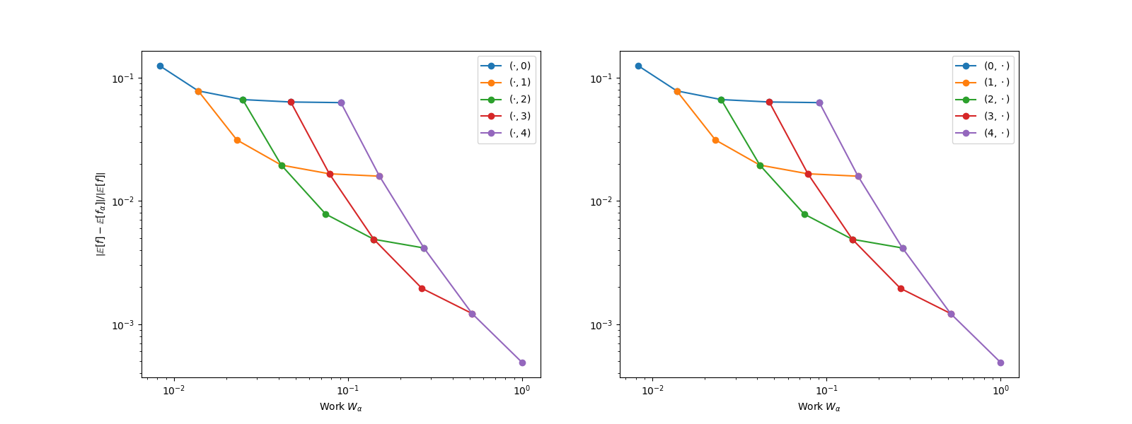
The left plots depicts the convergence of the estimated integral as \(n_1\) is increased for varying values of \(n_1\) and vice-versa for the right plot. These plots confirm that the Integrator converges as the expected linear rate. Until the error introduced by fixing the other configuration variables dominates.

We can also generate similar plots for methods used to solve parameterized partial differential equations. I the following we will assess convergence of a spectral collocation method used to solve the transient advection diffusion equation on a rectangle (see setup_multi_index_advection_diffusion_benchmark()).

from pyapprox.benchmarks import setup_benchmark
np.random.seed(1)
final_time = 0.5
time_scenario = {
    "final_time": final_time,
    # "butcher_tableau": "im_beuler1",
    "butcher_tableau": "im_crank2",
    "deltat": final_time/100,  # will be overwritten
    "init_sol_fun": None,
    # "init_sol_fun": partial(full_fun_axis_1, 0),
    "sink": None  # [50, 0.1, [0.75, 0.75]]
}

N = 8
config_values = [2*np.arange(1, N+2)+5, 2*np.arange(1, N+2)+5,
                 final_time/((2**np.arange(1, N+2)+40))]
# values of kle stdev and mean before exponential is taken
log_kle_mean_field = np.log(0.1)
log_kle_stdev = 1
benchmark = setup_benchmark(
    "multi_index_advection_diffusion", kle_nvars=3, kle_length_scale=1,
    kle_stdev=log_kle_stdev,
    time_scenario=time_scenario, config_values=config_values,
    vel_vec=[0.2, -0.2], source_loc=[0.5, 0.5], source_amp=1,
    kle_mean_field=log_kle_mean_field)

First plot the evolution of the PDE for a realization of the model inputs

import torch
from pyapprox.pde.autopde.mesh import generate_animation
model = benchmark.fun.base_model._model_ensemble.functions[0]
sample = torch.as_tensor(benchmark.variable.rvs(1)[:, 0])
model._set_random_sample(sample)
init_sol = model._get_init_sol(sample)
sols, times = model._fwd_solver.solve(
    init_sol, 0, model._final_time,
    newton_kwargs=model._newton_kwargs, verbosity=0)
ani = generate_animation(
    model._fwd_solver.physics.mesh, sols, times,
    filename=None, maxn_frames=100, duration=2)
import matplotlib.animation as animation
ani.save('ad-sol.gif', writer=animation.ImageMagickFileWriter(),
         dpi=100)

Once Loop Reflect

Now perform a convgernce study

validation_levels = np.full(3, N)
coarsest_levels = np.full(3, 0)
finest_levels = np.full(3, N-4)
if final_time is None:
    validation_levels = validation_levels[:2]
    coarsest_levels = coarsest_levels[:2]
convergence_data = run_convergence_study(
    benchmark.fun, benchmark.variable, validation_levels,
    benchmark.get_num_degrees_of_freedom, benchmark.config_var_trans,
    num_samples=1, coarsest_levels=coarsest_levels,
    finest_levels=finest_levels)
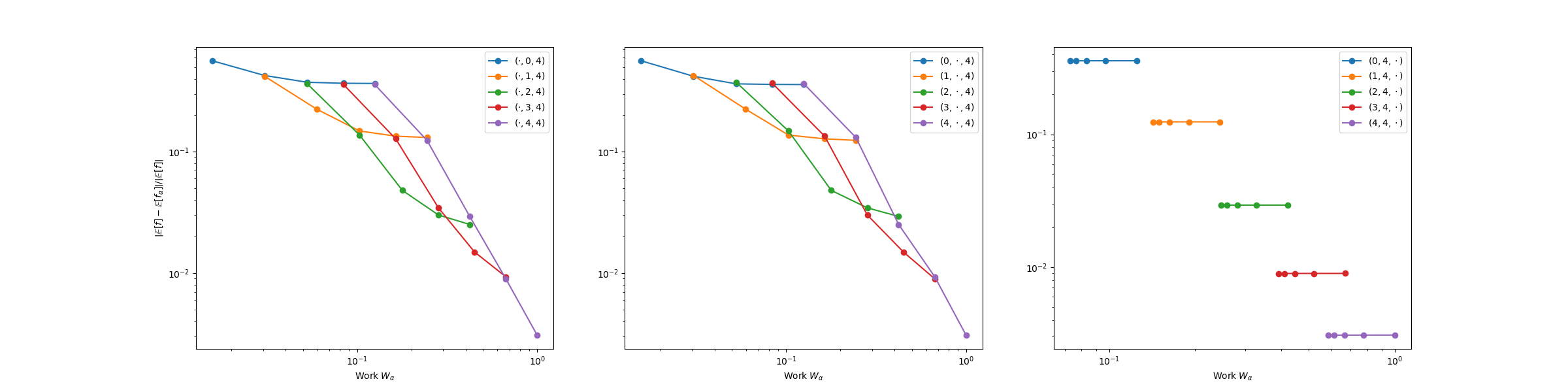
_ = plot_convergence_data(convergence_data, cost_type="ndof")

Note when because the benchmark fun is run using multiprocessing.Pool The .py script of this tutorial cannot be run with max_eval_concurrency > 1 via the shell command using python plot_pde_convergence.py because Pool must be called inside

if __name__ == '__main__':