Two model Approximate Control Variate Monte Carlo

This tutorial builds upon Two Model Control Variate Monte Carlo and describes how to implement and deploy approximate control variate Monte Carlo (ACVMC) [GGEJJCP2020] sampling to compute expectations of model output from a single low-fidelity models with an unknown statistic.

CVMC is often not useful for practical analysis of numerical models because typically the statistic of the lower fidelity model is unknown and the cost of the lower fidelity model is non trivial. These two issues can be overcome by using approximate control variate Monte Carlo.

Let the cost of the high fidelity model per sample be \(C_\alpha\) and let the cost of the low fidelity model be \(C_\kappa\). A two-model ACV estimators uses \(N\) samples to estimate \(Q_{\alpha}(\rvset_N)\) and \(Q_{\kappa}(\rvset_N)\) another set of samples \(\rvset_{rN}\) to estimate the exact statistic \(Q_{\alpha}\) via

\[Q_{{\alpha}}^{\text{ACV}}(\rvset_N, \rvset_{rN})=Q_{\alpha}(\rvset_N) + \eta \left( Q_{\kappa}(\rvset_N) -Q_{\kappa}(\rvset_{rN}) \right)\]

As with CV, the third term \(Q_{\kappa}(\rvset_{rN})\) is used to ensure the the ACV estimator is unbiased, but unlike CV it is estimated using a set of samples, rather than being assumed known.

In the following we will focus on the estimation of \(Q_\alpha=\mean{f_\alpha}\) with two models. Future tutorials will show how ACV can be used to compute other statistics and with more than two models.

First, an ACV estimator is unbiased

\[\begin{split}\mean{Q_{{\alpha}}^{\text{ACV}}(\rvset_N, \rvset_{rN})}&=\mean{Q_{\alpha}(\rvset_N)} + \mean{\eta \left( Q_{\kappa}(\rvset_N) -Q_{\kappa}(\rvset_{rN}) \right)}\\ &=\mean{f_\alpha}+\eta\left(\mean{Q_{\kappa}(\rvset_N)} -\mean{Q_{\kappa}(\rvset_{rN})}\right)\\ &=\mean{f_\alpha}.\end{split}\]

so the MSE of an ACV estimator is equal to the variance of the estimator (when estimating a single statistic).

The ACV estimator variance is dependent on the size and structure of the two sample sets \(\rvset_N, \rvset_{rN}.\) For ACV to reduce the variance of a single model MC estimator \(\rvset_N\subset\rvset_{rN}\). That is we evaluate \(f_\alpha, f_\kappa\) at a common set of samples and evaluate \(f_\kappa\) at an additional \(rN-N\) samples. For convenience we write the number of samples used to evaluate \(f_\kappa\) as \(rN, r> 1\) so that

\[Q_{\kappa}(\rvset_{rN})=\frac{1}{rN}\sum_{i=1}^{rN}f_{\kappa}^{(i)}.\]

With this sampling scheme we have

\[\begin{split}Q_{\kappa}(\rvset_N) - Q_{\kappa}(\rvset_{rN}) &=\frac{1}{N}\sum_{i=1}^N f_{\kappa}^{(i)}-\frac{1}{rN}\sum_{i=1}^{rN}f_{\kappa}^{(i)}\\ &=\frac{1}{N}\sum_{i=1}^N f_{\kappa}^{(i)}-\frac{1}{rN}\sum_{i=1}^{N}f_{\kappa}^{(i)}-\frac{1}{rN}\sum_{i=N}^{rN}f_{\kappa}^{(i)}\\ &=\frac{r-1}{rN}\sum_{i=1}^N f_{\kappa}^{(i)}-\frac{1}{rN}\sum_{i=N}^{rN}f_{\kappa}^{(i)}.\end{split}\]

Using the above expression yields

\[\begin{split}\var{\left( Q_{\kappa}(\rvset_N) - Q_{\kappa}(\rvset_{rN})\right)}&=\mean{\left(\frac{r-1}{rN}\sum_{i=1}^N f_{\kappa}^{(i)}-\frac{1}{rN}\sum_{i=N}^{rN}f_{\kappa}^{(i)}\right)^2}\\ &=\frac{(r-1)^2}{r^2N^2}\sum_{i=1}^N \var{f_{\kappa}^{(i)}}+\frac{1}{r^2N^2}\sum_{i=N}^{rN}\var{f_{\kappa}^{(i)}}\\ &=\frac{(r-1)^2}{r^2N^2}N\var{f_{\kappa}}+\frac{1}{r^2N^2}(r-1)N\var{f_{\kappa}}\\ %&=\left(\frac{(r-1)^2}{r^2N}+\frac{(r-1)}{r^2N}\right)\var{f_{\kappa}}\\ &=\frac{r-1}{r}\frac{\var{f_{\kappa}}}{N},\end{split}\]

where we have used the fact that since the samples used in the first and second term on the first line are not shared, the covariance between these terms is zero. Also we have

\[\covar{Q_{\alpha}(\rvset_N)}{\left( Q_{\kappa}(\rvset_N) - Q_{\kappa}(\rvset_{rN})\right)}=\covar{\frac{1}{N}\sum_{i=1}^N f_{\alpha}^{(i)}}{\frac{r-1}{rN}\sum_{i=1}^N f_{\kappa}^{(i)}-\frac{1}{rN}\sum_{i=N}^{rN}f_{\kappa}^{(i)}}\]

The correlation between the estimators \(\frac{1}{N}\sum_{i=1}^{N}Q_{\alpha}\) and \(\frac{1}{rN}\sum_{i=N}^{rN}Q_{\kappa}\) is zero because the samples used in these estimators are different for each model. Thus

\[\begin{split} \covar{Q_{\alpha}(\rvset_N)}{\left( Q_{\kappa}(\rvset_N) - Q_{\kappa}(\rvset_{rN})\right)} &=\covar{\frac{1}{N}\sum_{i=1}^N f_{\alpha}^{(i)}}{\frac{r-1}{rN}\sum_{i=1}^N f_{\kappa}^{(i)}}\\ &=\frac{r-1}{r}\frac{\covar{f_{\alpha}}{f_{\kappa}}}{N}\end{split}\]

Recalling the variance reduction of the CV estimator using the optimal \(\eta\) is

\[\begin{split}\gamma &= 1-\frac{\covar{Q_{\alpha}(\rvset_N)}{\left( Q_{\kappa}(\rvset_N) - Q_{\kappa}(\rvset_{rN})\right)}^2}{\var{\left( Q_{\kappa}(\rvset_N) - Q_{\kappa}(\rvset_{rN})\right)}\var{Q_{\alpha}(\rvset_N)}}\\ &=1-\frac{N^{-2}\frac{(r-1)^2}{r^2}\covar{f_{\alpha}}{f_{\kappa}}}{N^{-1}\frac{r-1}{r}\var{f_{\kappa}}N^{-1}\var{f_{\alpha}}}\\ &=1-\frac{r-1}{r}\corr{f_{\alpha}}{f_{\kappa}}^2\end{split}\]

which is found when

\[\begin{split} \eta&=-\frac{\covar{Q_{\alpha}(\rvset_N)}{\left( Q_{\kappa}(\rvset_N) - Q_{\kappa}(\rvset_{rN})\right)}}{\var{\left( Q_{\kappa}(\rvset_N) - Q_{\kappa}(\rvset_{rN)}\right)}}\\ &=-\frac{N^{-1}\frac{r-1}{r}\covar{f_{\alpha}}{f_{\kappa}}}{N^{-1}\frac{r-1}{r}\var{f_{\kappa}}}\\ &=-\frac{\covar{f_{\alpha}}{f_{\kappa}}}{\var{f_{\kappa}}}\end{split}\]

Finally, letting \(C_\alpha\) and \(C_\kappa\) denote the computational cost of simluating the models \(f_\alpha\) and \(f_\kappa\) at one sample, respectively, the cost of computing a two model ACV estimator is

\[C^\mathrm{ACV} = NC_\alpha + rNC_\kappa.\]

The following code can be used to investigate the properties of a two model ACV estimator.

First setup the problem and compute an ACV estimate of \(\mean{f_0}\)

import numpy as np
import matplotlib.pyplot as plt

from pyapprox.benchmarks import setup_benchmark
from pyapprox.util.visualization import mathrm_label

np.random.seed(1)
shifts = [.1, .2]
benchmark = setup_benchmark(
    "tunable_model_ensemble", theta1=np.pi/2*.95, shifts=shifts)
model = benchmark.fun
exact_integral_f0 = benchmark.mean[0]

Now initialize the estimator

from pyapprox.multifidelity.factory import (
    get_estimator, numerically_compute_estimator_variance, multioutput_stats)
# The benchmark has three models, so just extract data for first two models
costs = benchmark.fun.costs()[:2]
stat = multioutput_stats["mean"](benchmark.nqoi)
stat.set_pilot_quantities(benchmark.covariance[:2, :2])
est = get_estimator("gis", stat, costs)

Set the number of samples in the two independent sample partitions to \(M=10\) and \(N=100\). For reasons that will become clear in later tuotials the code requires the specification of the number of samples in each independent set of samples i.e. in \(\mathcal{Z}_N\) and \(\mathcal{Z}_N\cup\mathcal{Z}_N\)

nhf_samples = 10   # The value N
npartition_ratios = [9]  # Defines the value of M-N
target_cost = (
    nhf_samples*costs[0]+(1+npartition_ratios[0])*nhf_samples*costs[1])
#We set using a private function (starts with an underscore) because in practice
#the number of samples should be optimized and set with est.allocate samples
est._set_optimized_params(npartition_ratios, target_cost)

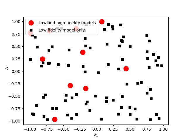
Now lets plot the samples assigned to each model.

samples_per_model = est.generate_samples_per_model(benchmark.variable.rvs)
print(est._rounded_npartition_samples)
samples_shared = (
    samples_per_model[0][:, :int(est._rounded_npartition_samples[0])])
samples_lf_only = (
    samples_per_model[1][:, int(est._rounded_npartition_samples[0]):])

fig, ax = plt.subplots()
ax.plot(samples_shared[0, :], samples_shared[1, :], 'ro', ms=12,
        label=mathrm_label("Low and high fidelity models"))
ax.plot(samples_lf_only[0, :], samples_lf_only[1, :], 'ks',
        label=mathrm_label("Low fidelity model only"))
ax.set_xlabel(r'$z_1$')
ax.set_ylabel(r'$z_2$', rotation=0)
_ = ax.legend(loc='upper left')

tensor([10., 90.])

The high-fidelity model is only evaluated on the red dots.

Now lets use both sets of samples to construct the ACV estimator

values_per_model = [benchmark.funs[ii](samples_per_model[ii])
                    for ii in range(len(samples_per_model))]
acv_mean = est(values_per_model)

print('MC difference squared =', (
    values_per_model[0].mean()-exact_integral_f0)**2)
print('ACVMC difference squared =', (acv_mean-exact_integral_f0)**2)

MC difference squared = [0.16633083]
ACVMC difference squared = [0.01069783]

Note here we have arbitrarily set the number of high fidelity samples \(N\) and the ratio \(r\). In practice one should choose these in one of two ways: (i) for a fixed budget choose the free parameters to minimize the variance of the estimator; or (ii) choose the free parameters to achieve a desired MSE (variance) with the smallest computational cost.

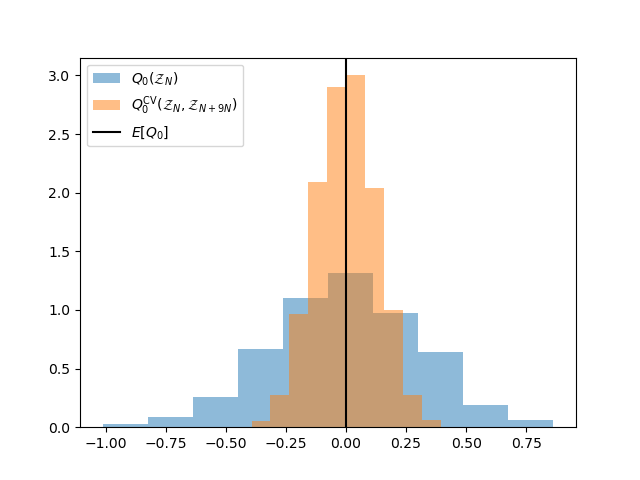
Now plot the distribution of this estimators and compare it against a single-fidelity MC estimator of the same target cost

nhf_samples = 10
ntrials = 1000
npartition_ratios = np.array([9])
target_cost = (
    nhf_samples*costs[0]+(1+npartition_ratios[0])*nhf_samples*costs[1])
est._set_optimized_params(npartition_ratios, target_cost)
numerical_var, true_var, means = (
    numerically_compute_estimator_variance(
        benchmark.funs[:2], benchmark.variable, est, ntrials, 1,
        return_all=True))[2:5]


sfmc_est = get_estimator("mc", stat, costs)
sfmc_est.allocate_samples(target_cost)
sfmc_means = (
    numerically_compute_estimator_variance(
        benchmark.funs[:1], benchmark.variable, sfmc_est, ntrials,
        return_all=True))[5]

fig, ax = plt.subplots()
ax.hist(sfmc_means, bins=ntrials//100, density=True, alpha=0.5,
        label=r'$Q_{0}(\mathcal{Z}_N)$')
ax.hist(means, bins=ntrials//100, density=True, alpha=0.5,
        label=r'$Q_{0}^\mathrm{CV}(\mathcal{Z}_N,\mathcal{Z}_{N+%dN})$' % (
            npartition_ratios[0]))
ax.axvline(x=0, c='k', label=r'$E[Q_0]$')
_ = ax.legend(loc='upper left')

Now compare what happens as we increase the number of low-fidelity samples. Eventually, adding more low-fidelity samples will no-longer reduce the ACV estimator variance. Asymptotically, the accuracy will approach the accuracy that can be obtained by the CV estimator that assumes the mean of the low-fidelity model is known. To reduce the variance further the number of high-fidelity samples must be increased. When this is done more low-fidelity samples can be added before their impact stagnates.

fig, ax = plt.subplots()
ax.hist(means, bins=ntrials//100, density=True, alpha=0.5,
        label=r'$Q_{0}^\mathrm{CV}(\mathcal{Z}_N,\mathcal{Z}_{N+%dN})$' % (
            npartition_ratios[0]))

npartition_ratios = np.array([99])
target_cost = (
    nhf_samples*costs[0]+(1+npartition_ratios[0])*nhf_samples*costs[1])
est._set_optimized_params(npartition_ratios, target_cost)
numerical_var, true_var, means = (
    numerically_compute_estimator_variance(
        benchmark.funs[:2], benchmark.variable, est, ntrials,
        return_all=True))[2:5]
ax.hist(means, bins=ntrials//100, density=True, alpha=0.5,
        label=r'$Q_{0}^\mathrm{CV}(\mathcal{Z}_N,\mathcal{Z}_{N+%dN})$' % (
            npartition_ratios[0]))
ax.axvline(x=0, c='k', label=r'$E[Q_0]$')
_ = ax.legend(loc='upper left')

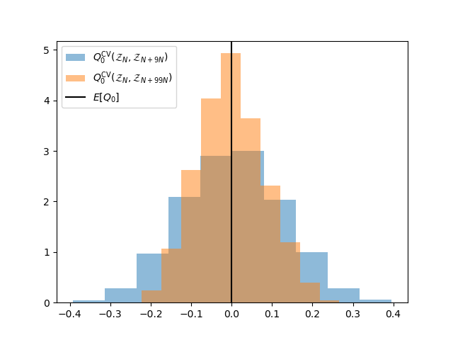
Note the two ACV estimators do not have the same computational cost. They are compared solely to show the impact of increasing the number of low-fidelity samples.

References

[GGEJJCP2020]

A generalized approximate control variate framework for multifidelity uncertainty quantification, Journal of Computational Physics, 408:109257, 2020.