Approximate Control Variate Monte Carlo

This tutorial builds upon Two model Approximate Control Variate Monte Carlo, Multi-level Monte Carlo, and Multi-fidelity Monte Carlo. MLMC and MFMC are two approaches which can utilize an ensemble of models of vary cost and accuracy to efficiently estimate the expectation of the highest fidelity model. In this tutorial we introduce a general framework for ACVMC when using two or more models to estimate vector-valued statistics.

The approximate control variate estimator of a vector-valued statistic \(\mat{Q}_0\in\reals^{S}\) that uses \(M\) lower fidelity models is

\[\begin{split}\mat{Q}_{\text{ACV}}(\rvset_0,\rvset_1^*,\rvset_1,\ldots,\rvset^*_M, \rvset_M) &= \mat{Q}_{0}(\rvset_0)+\begin{bmatrix}\eta_{1,1} & \cdots &\eta_{1, SM}\\ \eta_{2,1} & \cdots &\eta_{2, SM}\\ \vdots\\ \eta_{S,1} & \cdots &\eta_{S, SM} \end{bmatrix}\begin{bmatrix} \mat{Q}_{1}(\rvset_1^*)-\mat{Q}_{1}(\rvset_1) \\ \mat{Q}_{2}(\rvset_2^*)-\mat{Q}_{2}(\rvset_2) \\ \vdots \\ \mat{Q}_{M}(\rvset_M^*)-\mat{Q}_{M}(\rvset_M)\end{bmatrix}\in\reals^{S}\end{split}\]

or in more compact notation

\[\begin{split}\mat{Q}_{\text{ACV}}(\rvset_\text{ACV})&=\mat{Q}_{0}(\rvset_0)+\mat{\eta}\mat{\Delta}(\rvset_{\Delta}), \quad \mat{\Delta}(\rvset_\Delta) = \begin{bmatrix}\mat{\Delta}_1(\rvset_1^*, \rvset_1)\\ \vdots\\ \mat{\Delta}_M(\rvset_M^*,\rvset_M)\end{bmatrix}\in\reals^{SM}, \quad \mat{\eta}\in\reals^{S\times SM},\end{split}\]

where the entries of \(\mat{\eta}\) are called control variate weights, \(\rvset_\Delta=\{\rvset_1^*, \rvset_1, \ldots, \rvset_M^*, \rvset_M\}\), and \(\rvset_\text{ACV}=\{\rvset_0, \rvset_\Delta\}\).

Here \(\mat{\eta}=[\eta_1,\ldots,\eta_M]^T\), \(\mat{\Delta}=[\Delta_1,\ldots,\Delta_M]^T\), and \(\rvset_{\alpha}^*\), \(\rvset_{\alpha}\) are sample sets that may or may not be disjoint. Specifying the exact nature of these sets, including their cardinality, can be used to design different ACV estimators which will discuss later.

This estimator is constructed by evaluating each model at two sets of samples \(\rvset_{\alpha}^*=\{\rv^{(n)}\}_{n=1}^{N_{\alpha^*}}\) and \(\rvset_{\alpha}=\{\rv^{(n)}\}_{n=1}^{N_\alpha}\) where some samples may be shared between sets such that in some cases \(\rvset_{\alpha}^*\cup\rvset_{\beta}\neq \emptyset\).

For any \(\mat{\eta}(\rvset_\text{ACV})\), the covariance of the ACV estimator is

\[\var{\mat{Q}^{\text{ACV}}} = \var{\mat{Q}_{0}}+\mat{\eta}\covar{\mat{\Delta}}{\mat{\Delta}}\mat{\eta}^\top+\mat{\eta}\covar{\mat{\Delta}}{\mat{Q}_0}+\covar{\mat{\Delta}}{\mat{Q}_0}\mat{\eta}^\top, \qquad\in\reals^{S\times S}\]

The control variate weights that minimize the determinant of the ACV estimator covariance are

\[\mat{\eta} = -\covar{\mat{\Delta}}{\mat{\Delta}}^{-1}\covar{\mat{\Delta}}{\mat{Q}_0}\]

The ACV estimator covariance using the optimal control variate weights is

\[\covar{\mat{Q}_{\text{ACV}}}{\mat{Q}_{\text{ACV}}}(\rvset_\text{ACV})=\covar{\mat{Q}_0}{ \mat{Q}_0}-\covar{\mat{Q}_0}{\mat{\Delta}}\covar{\mat{\Delta}}{\mat{\Delta}}^{-1}\covar{\mat{Q}_0}{\mat{\Delta}}^\top\]

Computing the ACV estimator covariance requires computing \(\covar{\mat{Q}_0}{\mat{\Delta}}\text{ and} \covar{\mat{\Delta}}{\mat{\Delta}}\).

First

\[\begin{split}\covar{\mat{\Delta}}{\mat{\Delta}} = \begin{bmatrix}\covar{\mat{\Delta}_1}{\mat{\Delta}_1} & \covar{\mat{\Delta}_1}{\mat{\Delta}_2} & \cdots & \covar{\mat{\Delta}_1}{\mat{\Delta}_M}\\ \covar{\mat{\Delta}_2}{\mat{\Delta}_1} & \covar{\mat{\Delta}_1}{\mat{\Delta}_2} & & \vdots\\ \vdots & & \ddots & \vdots \\ \covar{\mat{\Delta}_M}{\mat{\Delta}_1} & \cdots & \cdots & \covar{\mat{\Delta}_M}{\mat{\Delta}_M} \end{bmatrix}\end{split}\]

and second

\[\covar{\mat{Q}_0}{\mat{\Delta}} = [\covar{\mat{Q}_0}{\mat{\Delta}_1}, \ldots, \covar{\mat{Q}_0}{\mat{\Delta}_M}]\]

where

\[\covar{\mat{Q}_0}{\mat{\Delta}_\alpha} = \covar{\mat{Q}_0(\rvset_0)}{\mat{\Delta}_\alpha(\rvset_\alpha^*)}-\covar{\mat{Q}_0(\rvset_0)}{\mat{\Delta}_\alpha(\rvset_\alpha)}]\]

When estimating the statistics in Monte Carlo Quadrature: Beyond Mean Estimation the above coavariances involving \(\Delta\) can be computed using the formula in Delta-Based Covariance Formulas For Approximate Control Variates.

The variance of an ACV estimator is dependent on how samples are allocated to the sets \(\rvset_\alpha,\rvset_\alpha^*\), which we call the sample allocation \(\mathcal{A}\). Specifically, \(\mathcal{A}\) specifies: the number of samples in the sets \(\rvset_\alpha,\rvset_\alpha^*, \forall \alpha\), denoted by \(N_\alpha\) and \(N_{\alpha^*}\), respectively; the number of samples in the intersections of pairs of sets, that is \(N_{\alpha\cap\beta} =|\rvset_\alpha \cap \rvset_\beta|\), \(N_{\alpha^*\cap\beta} =|\rvset_\alpha^* \cap \rvset_\beta|\), \(N_{\alpha^*\cap\beta^*} =|\rvset_\alpha^* \cap \rvset_\beta^*|\); and the number of samples in the union of pairs of sets \(N_{\alpha\cup\beta} = |\rvset_\alpha\cup \rvset_\beta|\) and similarly \(N_{\alpha^*\cup\beta}\), \(N_{\alpha^*\cup\beta^*}\). Thus, finding the best ACV estimator can be theoretically be found by solving the constrained non-linear optimization problem

\[\min_{\mathcal{A}\in\mathbb{A}}\mathrm{Det}\left[\covar{\mat{Q}_{\text{ACV}}}{\mat{Q}_{\text{ACV}}}\right](\mathcal{A}) \qquad \mathrm{s.t.} \qquad C(\mat{c},\tilde{\mathcal{A}})\le C_\mathrm{max},\]

Here, \(\tilde{\mathcal{A}}\) is the set of all possible sample allocations, and given the computational costs of evaluating each model once \(c^\top=[c_0, c_1, \ldots, c_M]\), the constraint ensures that the computational cost of computing the ACV estimator

\[C(\mat{c},\mathcal{A})=\sum_{\alpha=0}^M N_{\alpha^*\cup\alpha}c_\alpha\]

is smaller than a user-specified computational budget \(C_\mathrm{max}\).

Unfortunately, to date, no method has been devised to solve the above optimization problem for all possible allocations \(\tilde{\mathcal{A}}\). Consequently, all existing ACV methods restrict the optimization space to \(\mathcal{A}\subset\tilde{\mathcal{A}}\). These restricted search spaces are formulated in terms of a set of \(M+1\) independent sample partitions \(\mathcal{P}_m\) that contain \(p_m\) samples drawn indepedently from the PDF of the random variable \(\rv\). Each subset \(\rvset_\alpha\) is then assumed to consist of a combinations of these indepedent partitions. ACV methods encode the relationship between the sets \(\rvset_\alpha\) and \(\mathcal{P}_m\) via allocation matrices \(\mat{A}\). For example, the allocation matrix used by MFMC, which is an ACV method, when applied to three models is given by

\[\begin{split}\mat{A} = \begin{bmatrix} 0 & 1 & 1 & 1 & 1 & 1 & 1 & 1\\ 0 & 0 & 0 & 1 & 1 & 1 & 1 & 1\\ 0 & 0 & 0 & 0 & 0 & 1 & 1 & 1\\ 0 & 0 & 0 & 0 & 0 & 0 & 0 & 1 \end{bmatrix}\end{split}\]

An entry of one indicates in the ith row of the jth column indicates that the ith independent partition \(\mathcal{P}_i\) is used in the corresponding set \(\rvset_j\) if j is odd or \(\rvset_j^*\) if j is even. The first column will always only contain zeros because the set \(\rvset_0^*\) is never used by ACV estimators.

Once an allocation matrix is specified, the optimal sample allocation can be obtained by optimizing the number of samples in each partition \(\mat{p}=[p_0,\ldots,p_M]^\top\), that is

\[\min_{\mat{p}}\mathrm{Det}\left[\covar{\mat{Q}_{\text{ACV}}}{\mat{Q}_{\text{ACV}}}\right](\mat{p}; \mat{A}) \qquad \mathrm{s.t.} \qquad C(\mat{c},\mat{p};\mat{A})\le C_\mathrm{max},\]

The following tutorials introduce different ACV methods and their allocation matrices that have been introduced in the literature.

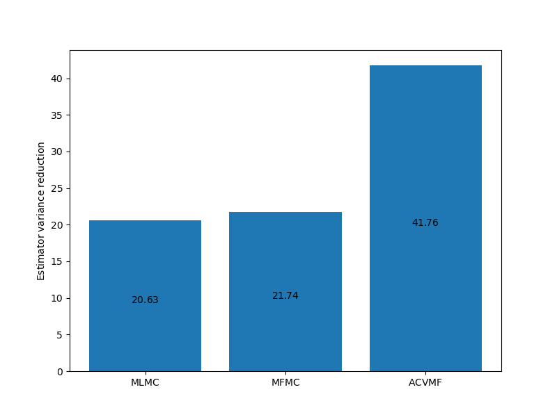
The following compares the estimator variances of three different ACV estimators. No one estimator type is best for all problems. Consequently for any given problem all possible estimators should be constructed. This requires estimates of the model covariance using a pilot study see Pilot Studies

import numpy as np
import matplotlib.pyplot as plt

from pyapprox.util.visualization import mathrm_labels
from pyapprox.benchmarks import setup_benchmark
from pyapprox.multifidelity.factory import (
    get_estimator, compare_estimator_variances, multioutput_stats)
from pyapprox.multifidelity.visualize import (
    plot_estimator_variance_reductions)

np.random.seed(1)
benchmark = setup_benchmark("polynomial_ensemble")
model = benchmark.fun
cov = model.get_covariance_matrix()
nmodels = cov.shape[0]
target_costs = np.array([1e2], dtype=int)
costs = np.asarray([10**-ii for ii in range(nmodels)])
model_labels = [r'$f_0$', r'$f_1$', r'$f_2$', r'$f_3$', r'$f_4$']

stat = multioutput_stats["mean"](benchmark.nqoi)
stat.set_pilot_quantities(cov)
estimators = [
    get_estimator("mlmc", stat, costs),
    get_estimator("mfmc", stat, costs),
    get_estimator("gmf", stat, costs,
                  recursion_index=np.zeros(nmodels-1, dtype=int))]
est_labels = mathrm_labels(["MLMC", "MFMC", "ACVMF"])
optimized_estimators = compare_estimator_variances(
    target_costs, estimators)

axs = [plt.subplots(1, 1, figsize=(8, 6))[1]]

# get estimators for target cost = 100
ests_100 = [ests[0] for ests in optimized_estimators]
_ = plot_estimator_variance_reductions(
    ests_100, est_labels, axs[0])

Video

Click on the image below to view a video tutorial on approximate control variate Monte Carlo quadrature