Sparse Grids

The number of model evaluations required by tensor product interpolation grows exponentitally with the number of model inputs. This tutorial introduces sparse grids [BNR2000], [BG2004] which can be used to overcome the so called curse of dimensionality faced by tensor-product methods.

Sparse grids approximate a model (function) \(f_\alpha\) with \(D\) inputs \(z=[z_1,\ldots,z_D]^\top\) as a linear combination of low-resolution tensor product interpolantsm that is

\[f_{\alpha, \mathcal{I}}(z) = \sum_{\beta\in \mathcal{I}} c_\beta f_{\alpha,\beta}(z),\]

where \(\beta=[\beta_1,\ldots,\beta_D]\) is a multi-index controlling the number of samples in each dimension of the tensor-product interpolants, and the index set \(\mathcal{I}\) controls the approximation accuracy and data-efficiency of the sparse grid. If the set \(\mathcal{I}\) is downward closed, that is

\[\gamma \le \beta \text{ and } \beta \in \mathcal{I} \implies \gamma \in \mathcal{I},\]

where the \(\le\) is applied per entry, then the (Smolyak) coefficients of the sparse grid are given by

\[\sum_{i\in [0,1]^D, \alpha+i\in \mathcal{I}} (-1)^{\lVert i \rVert_1}.\]

While any tensor-product approximation can be used with sparse grids, e.g. based on piecewise-polynomials or splines, in this tutorial we will build sparse grids with Lagrange polynomials (see Tensor-product Interpolation).

The following code compares a tensor-product interpolant with a level-\(l\) isotropic sparse grid which sets

\[\mathcal{I}(l)=\{\beta \mid (\max(0,l-1)\le \lVert\beta\rVert_1\le l+D-2\}, \quad l\ge 0\]

which leads to a simpler expression for the coefficients

\[c_\beta = (-1)^{l-\lvert\beta\rvert_1} {D-1\choose l-\lvert\beta\rvert_1}.\]

First import the necessary modules and define the function we will approximate and its variable \(\rv\).

\[f(\rv) = \cos(\pi\rv_1)\cos(\pi\rv_2/2)\]

import copy
import numpy as np
from scipy import stats
from pyapprox.util.visualization import get_meshgrid_function_data, plt
from pyapprox.variables.joint import IndependentMarginalsVariable
from pyapprox.surrogates.approximate import adaptive_approximate
from pyapprox.surrogates.interp.adaptive_sparse_grid import (
    tensor_product_refinement_indicator, isotropic_refinement_indicator,
    variance_refinement_indicator)
from pyapprox.surrogates.orthopoly.quadrature import (
    clenshaw_curtis_in_polynomial_order, clenshaw_curtis_rule_growth)
from pyapprox.util.utilities import nchoosek
from pyapprox.benchmarks import setup_benchmark

variable = IndependentMarginalsVariable([stats.uniform(-1, 2)]*2)


def fun(zz):
    return (np.cos(np.pi*zz[0])*np.cos(np.pi*zz[1]/2))[:, None]

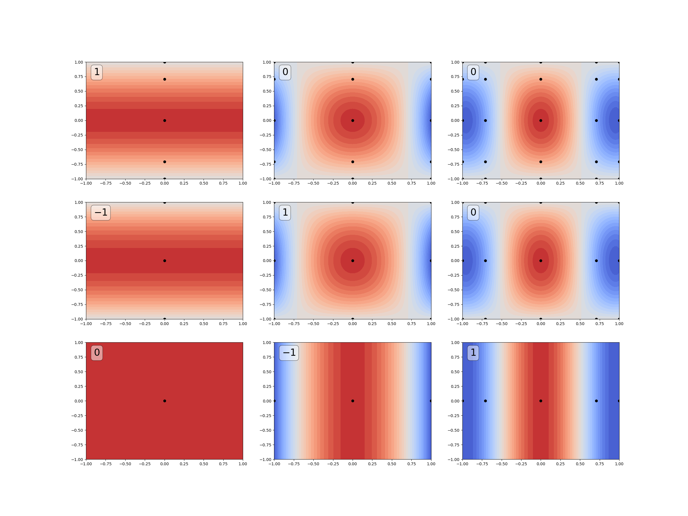
Now plot the tensor product interpolants and the Smolyak coefficients that make up the sparse grid. The coefficients are in the upper left corner of each subplot.

max_level = 2
fig, axs = plt.subplots(
    max_level+1, max_level+1, figsize=((max_level+1)*8, (max_level+1)*6))
ranges = variable.get_statistics("interval", 1.0).flatten()
univariate_quad_rule_info = [
    clenshaw_curtis_in_polynomial_order, clenshaw_curtis_rule_growth,
    None, None]


def build_tp(max_level_1d):
    tp = adaptive_approximate(
        fun, variable, "sparse_grid",
        {"refinement_indicator": tensor_product_refinement_indicator,
         "max_level_1d": max_level_1d,
         "univariate_quad_rule_info": univariate_quad_rule_info}).approx
    return tp


levels = np.linspace(-1.1, 1.1, 31)
text_props = dict(boxstyle='round', facecolor='white', alpha=0.5)
for ii in range(max_level+1):
    for jj in range(max_level+1):
        tp = build_tp([ii, jj])
        X, Y, Z_tp = get_meshgrid_function_data(tp, ranges, 71)
        ax = axs[max_level-jj][ii]
        ax.contourf(X, Y, Z_tp, levels=levels, cmap="coolwarm")
        ax.plot(*tp.samples, 'ko')
        coef = int((-1)**(max_level-(ii+jj))*nchoosek(
            variable.num_vars()-1, max_level-(ii+jj)))
        ax.text(0.05, 0.95, r"${:d}$".format(coef),
                transform=ax.transAxes, fontsize=24,
                verticalalignment='top', bbox=text_props)

Now compare the sparse grid with a tensor product interpolant of the same level.

fig, axs = plt.subplots(1, 3, figsize=(3*8, 6))
X, Y, Z_fun = get_meshgrid_function_data(fun, ranges, 51)
tp = adaptive_approximate(
    fun, variable, "sparse_grid",
    {"refinement_indicator": tensor_product_refinement_indicator,
     "max_level_1d": np.full(2, max_level),
     "univariate_quad_rule_info": univariate_quad_rule_info}).approx
sg = adaptive_approximate(
    fun, variable, "sparse_grid",
    {"refinement_indicator": isotropic_refinement_indicator,
     "max_level_1d": np.full(2, max_level),
     "univariate_quad_rule_info": univariate_quad_rule_info,
     "max_level": max_level}).approx
X, Y, Z_tp = get_meshgrid_function_data(tp, ranges, 51)
X, Y, Z_sg = get_meshgrid_function_data(sg, ranges, 51)
lb = np.min([Z_fun.min(), Z_tp.min(), Z_sg.min()])
ub = np.max([Z_fun.max(), Z_tp.max(), Z_sg.max()])
levels = np.linspace(lb, ub, 21)
im = axs[0].contourf(X, Y, Z_fun, levels=levels, cmap="coolwarm")
axs[1].contourf(X, Y, Z_tp, levels=levels, cmap="coolwarm")
axs[1].plot(*tp.samples, 'ko')
axs[2].contourf(X, Y, Z_sg, levels=levels, cmap="coolwarm")
axs[2].plot(*sg.samples, 'ko')
fig.subplots_adjust(right=0.9)
cbar_ax = fig.add_axes([0.9125, 0.125, 0.025, 0.75])
_ = fig.colorbar(im, cax=cbar_ax)
# plt.show()

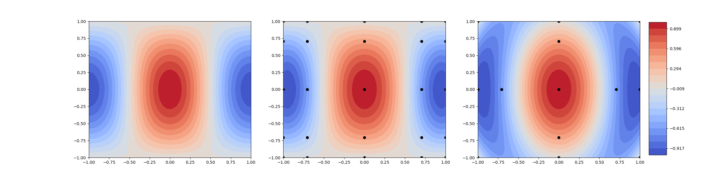
The sparse grid is slightly less accurate than the tensor product interpolant, but uses fewer points. There is no exact formula for the number of points in an isotropic sparse grid. The following code can be used to determine the number of points in a sparse grid of any dimension or level. The number of points is much smaller than the number of points in a tensor-product grid, for a given level \(l\).

def get_isotropic_sparse_grid_num_samples(
        nvars, max_level, univariate_quad_rule_info):
    """
    Get the number of points in an isotropic sparse grid
    """
    variable = IndependentMarginalsVariable([stats.uniform(-1, 2)]*nvars)

    def fun(xx):
        # a dummy function
        return np.ones((xx.shape[1], 1))
    sg = adaptive_approximate(
        fun, variable, "sparse_grid",
        {"refinement_indicator": isotropic_refinement_indicator,
         "max_level_1d": np.full(nvars, max_level),
         "univariate_quad_rule_info": univariate_quad_rule_info,
         "max_level": max_level, "verbose": 0, "max_nsamples": np.inf}).approx
    return sg.samples.shape[1]


sg_num_samples = [
    [get_isotropic_sparse_grid_num_samples(
        nvars, level, univariate_quad_rule_info) for level in range(5)]
    for nvars in [2, 3, 5]]
tp_num_samples = [
    [univariate_quad_rule_info[1](level)**nvars for level in range(5)]
    for nvars in [2, 3, 5]]
print("Growth of number of sparse grid points")
print(sg_num_samples)
print("Growth of number of tensor-product points")
print(tp_num_samples)

Growth of number of sparse grid points
[[1, 5, 13, 29, 65], [1, 7, 25, 69, 177], [1, 11, 61, 241, 801]]
Growth of number of tensor-product points
[[1, 9, 25, 81, 289], [1, 27, 125, 729, 4913], [1, 243, 3125, 59049, 1419857]]

For a function with \(r\) continous mixed-derivatives, the isotropic level-\(l\) sparse grid, based on 1D Clenshaw Curtis abscissa, with \(M_{\mathcal{I}(l)}\) points satisfies

\[\lVert f-f_{\mathcal{I}(l)}\rVert_{L^\infty}\le C_{D,r} M^{-r}_{\mathcal{I}(l)}(\log M_{\mathcal{I}(l)})^{(r+2)(D-1)+1}.\]

In contrast the tensor-product interpolant with \(M_l\) points satifies

\[\lVert f-f_{\mathcal{I}(l)}\rVert_{L^\infty}\le K_{D,r} M_l^{-r/D}.\]

The following code compares the convergence of sparse grids and tensor-product lagrange interpolants. A callback is used to compute the error as the level of the approximations increases

class IsotropicCallback():
    def __init__(self, validation_samples, validation_values, istp):
        self.level = -1
        self.errors = []
        self.nsamples = []
        self.validation_samples = validation_samples
        self.validation_values = validation_values
        self.istp = istp

    def __call__(self, approx):
        if self.istp:
            approx_level = approx.subspace_indices.max()
        else:
            approx_level = approx.subspace_indices.sum(axis=0).max()
        if self.level != approx_level:
            # only compute error when all subspaces of the current
            # approximation level are added to the sparse grid.
            # The number of sparse grid points will be slightly larger
            # than an isotoropic grid of level=approx_level because
            # points associated with active indies will be included here.
            self.level = approx_level
            self.nsamples.append(approx.samples.shape[1])
            approx_values = approx.evaluate_using_all_data(
                self.validation_samples)
            error = (np.linalg.norm(
                self.validation_values-approx_values) /
                     self.validation_samples.shape[1])
            self.errors.append(error)


def fun(xx):
    return np.exp(-0.05*(((xx+1)/2-0.5)**2).sum(axis=0))[:, None]


# do not go passed nvars,level = (4, 4) with clenshaw curtis rules
# do not go passed nvars,level = (5, 4) with Leja rules

nvars = 4
variable = IndependentMarginalsVariable([stats.uniform(-1, 2)]*nvars)
validation_samples = variable.rvs(1000)
validation_values = fun(validation_samples)

# switch to Leja quadrature rules with linear growth
# univariate_quad_rule_info = None

tp_max_level = 4
tp_callback = IsotropicCallback(validation_samples, validation_values, True)
tp = adaptive_approximate(
    fun, variable, "sparse_grid",
    {"refinement_indicator": tensor_product_refinement_indicator,
     "max_level_1d": np.full(nvars, tp_max_level),
     "univariate_quad_rule_info": univariate_quad_rule_info,
     "max_nsamples": np.inf, "callback": tp_callback,
     "verbose": 0}).approx
# compute error at final level
tp_callback.level = tp_max_level  # set so callback computes error
tp_callback(tp)

sg_max_level = 6
sg_callback = IsotropicCallback(validation_samples, validation_values, False)
sg = adaptive_approximate(
    fun, variable, "sparse_grid",
    {"refinement_indicator": isotropic_refinement_indicator,
     "max_level_1d": np.full(nvars, sg_max_level),
     "univariate_quad_rule_info": univariate_quad_rule_info,
     "max_level": sg_max_level, "max_nsamples": np.inf,
     "callback": sg_callback}).approx
# compute error at final level
sg_callback.level = sg_max_level  # set so callback computes error
sg_callback(sg)

ax = plt.subplots(1, 1, figsize=(8, 6))[1]
ax.loglog(tp_callback.nsamples, tp_callback.errors, '-o', label="TP")
ax.loglog(sg_callback.nsamples, sg_callback.errors, '--s', label="SG")
_ = ax.legend()
# plt.show()

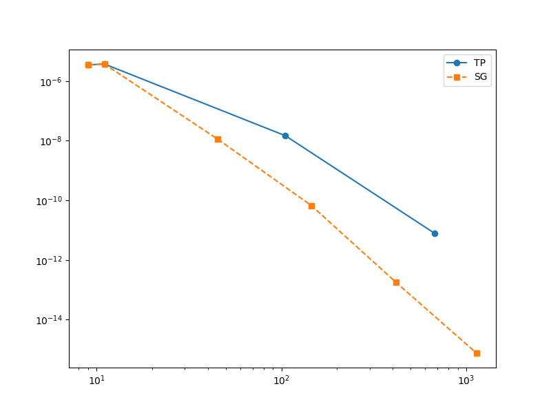
Experiment with changing nvars, e.g. try nvars = 2,3,4. Sparse grids become more effective as nvars increases.

So far we have used sparse grids based on Clenshaw-Curtis 1D quadrature rules. However other types of rules can be used. PyApprox also supports 1D Leja sequences [NJ2014] (see Adaptive Leja Sequences). Change univariate_quad_rule=None to use Leja rules and observe the difference in convergence.

Dimension adaptivity

The efficiency of sparse grids can be improved using methods [GG2003], [H2003] that construct the index set \(\mathcal{I}\) adaptively. This is the default behavior when using Pyapprox. The following applies the adaptive algorithm to an anisotropic function, where one variable impacts the function much more than the other.

Finding an efficient index set can be cast as an optimization problem. With this goal, let the difference in sparse grid error before and after the interpolant \(f_{\alpha,\beta}\) and the work from adding the new interpolant respectively be

\[\begin{align*}\Delta E_\beta = \lVert f_{\alpha, \mathcal{I}\cup\beta}-f_{\alpha, \mathcal{I}}\rVert && \Delta W_\beta = \lVert W_{\alpha, \mathcal{I}\cup\beta}-W_{\alpha, \mathcal{I}}\rVert\end{align*}\]

Then noting that the error in the sparse grid satisfies, we can formulate finding a quasi-optimal index set as a binary knapsack problem

\[\max \sum_{\beta}\Delta E_\beta\delta_\beta \text{ such that }\sum_{\beta}\Delta W_\beta\delta_\beta \le W_{\max},\]

for a total work budget \(W_{\max}\). The solution to this problem balances the computational work of adding a specific interpolant with the reduction in error that would be achieved.

The isotropic index set represents a solution to this knapsack problem under certain conditions on the smoothness of the function being approximated. However, for weaker conditions, finding optimal index sets by solving the knapsack problem is typically intractable. Consequently, we use a greedy adaptive procedure.

The algorithm begins with the index set \(\mathcal{I}=\{\beta\mid \beta=[0, \ldots, 0]\}\) then identifies, so called active indices, which are candidates for refinement. The active indices satisfy the downward closed admissibility criteria above. The function is evaluated at the points assoicated with the active indices and error indicators, similar to \(\Delta W_\beta\), are computed. The active index with the largest error indicator is then added to \(\mathcal{I}\) and the active set is updated. This procedure is repeated until and error threshold is met or a computational budget reached.

First set up the benchmark

benchmark = setup_benchmark(
    "genz", nvars=2, test_name='oscillatory', coeff=([2, 0.2], [0, 0]))

Now build a sparse grid using a callback that tracks important properties of the sparse grid and its adaptation.

class AdaptiveCallback():
    def __init__(self, validation_samples, validation_values):
        self.validation_samples = validation_samples
        self.validation_values = validation_values

        self.nsamples = []
        self.errors = []
        self.sparse_grids = []

    def __call__(self, approx):
        self.nsamples.append(approx.samples.shape[1])
        approx_values = approx.evaluate_using_all_data(
            self.validation_samples)
        error = (np.linalg.norm(
            self.validation_values-approx_values) /
                     self.validation_samples.shape[1])
        self.errors.append(error)
        self.sparse_grids.append(copy.deepcopy(approx))


validation_samples = benchmark.variable.rvs(100)
validation_values = benchmark.fun(validation_samples)
adaptive_callback = AdaptiveCallback(validation_samples, validation_values)
sg = adaptive_approximate(
    benchmark.fun, benchmark.variable, "sparse_grid",
    {"refinement_indicator": variance_refinement_indicator,
     "max_level_1d": np.inf,
     "univariate_quad_rule_info": None,
     "max_level": np.inf, "max_nsamples": 100,
     "callback": adaptive_callback}).approx

The following visualizes the adaptive algorithm.

The left plot depicts the multi-index of each tensor product interpolant. They gray boxes represent indices added to the sparse grid and the red boxes represent the active indices. The numbers in the boxes represent the Smolyak coefficients.

The middle plot shows the grid points associated with the gray boxes (black dots) and the grid points associated with the active indices (red dots).

The left plot depicts the sparse grid approximation at each iteration.

The sparse grid spends more points resolving the function variation in the horizontal direction, associated with the most sensitive function input.

from pyapprox.surrogates.interp.adaptive_sparse_grid import (
    plot_adaptive_sparse_grid_2d)

fig, axs = plt.subplots(1, 3, sharey=False, figsize=(3*8, 6))
ranges = benchmark.variable.get_statistics("interval", 1.0).flatten()
data = [get_meshgrid_function_data(sg, ranges, 51)
        for sg in adaptive_callback.sparse_grids]
Z_min = np.min([d[2] for d in data])
Z_max = np.max([d[2] for d in data])
levels = np.linspace(Z_min, Z_max, 21)
def animate(ii):
    [ax.clear() for ax in axs]
    sg = adaptive_callback.sparse_grids[ii]
    plot_adaptive_sparse_grid_2d(sg, axs=axs[:2])
    axs[2].contourf(*data[ii], levels=levels)
    axs[0].set_xlim([0, 10])
    axs[0].set_ylim([0, 10])

import matplotlib.animation as animation
ani = animation.FuncAnimation(
    fig, animate, interval=500,
    frames=len(adaptive_callback.sparse_grids), repeat_delay=1000)
ani.save("adaptive_sparse_grid.gif", dpi=100,
         writer=animation.ImageMagickFileWriter())

References

T. Gerstner and M. Griebel. Dimension-adaptive tensor-product quadrature. Computing (2003).
Total running time of the script: ( 0 minutes 32.437 seconds)