Gaussian processes

Gaussian processes (GPs) [RW2006] are an extremely popular tool for approximating multivariate functions from limited data. A GP is a distribution over a set of functions. Given a prior distribution on the class of admissible functions an approximation of a deterministic function is obtained by conditioning the GP on available observations of the function.

Constructing a GP requires specifying a prior mean \(m(\rv)\) and covariance kernel \(C(\rv, \rv^\star)\). The GP leverages the correlation between training samples to approximate the residuals between the training data and the mean function. In the following we set the mean to zero. The covariance kernel should be tailored to the smoothness of the class of functions under consideration. The matern kernel with hyper-parameters \(\theta=[\sigma^2,\ell^\top]^\top\) is a common choice.

\[C_\nu(\rv, \rv^\star; \theta)=\sigma^2 \frac{2^{1-\nu}}{\mathsf{\Gamma}(\nu)}\left(\frac{\sqrt{2\nu}d(\rv,\rv^\star; \ell)}{\ell}\right)^{\nu}K_{\nu}\left(\frac{\sqrt{2\nu}d(\rv,\rv^\star; \ell)}{\ell}\right).\]

Here \(d(\rv,\rv^\star; \ell)\) is the weighted Euclidean distance between two points parameterized by the vector hyper-parameters \(\ell=[\ell_1,\ldots,\ell_d]^\top\). The variance of the kernel is determined by \(\sigma^2\) and \(K_{\nu}\) is the modified Bessel function of the second kind of order \(\nu\) and \(\mathsf{\Gamma}\) is the gamma function. Note that the parameter \(\nu\) dictates for the smoothness of the kernel function. The analytic squared-exponential kernel can be obtained as \(\nu\to\infty\).

Given a kernel and mean function, a Gaussian process approximation assumes that the joint prior distribution of \(f\), conditional on kernel hyper-parameters \(\theta=[\sigma^2,\ell^\top]^\top\), is multivariate normal such that

\[f(\cdot) \mid \theta \sim \mathcal{N}\left(m(\cdot),C(\cdot,\cdot;\theta)+\epsilon^2I\right)\]

where \(\epsilon^2\) is the variance of the mean zero white noise in the observations.

The following plots realizations from the prior distribution of a Gaussian process at a set \(\mathcal{Z}\) of values of \(\rv\). Random realizations are drawn by taking the singular value decomposition of the kernel evaluated at the set of points \(\mathcal{Z}\), such that

\[USV = C(\mathcal{Z}, \mathcal{Z}),\]

where \(U, V\) are the left and right singular vectors and \(S\) are the singular values. The left singular vectors and singular values are then used to generate random realizations \(y\) using independent and identically distributed draws \(X\) from the multivariate standard Normal distribution \(\mathcal{N}(0, \V{I}_N)\), where \(\V{I}_N\) is the identity matrix of size \(N\), and \(N\) is the number of samples in \(\mathcal{Z}\). Specifically

\[y = US^{\frac{1}{2}}X.\]

Note the Cholesky decomposition could also be used instead of the singular value decomposition.

import numpy as np
import matplotlib.pyplot as plt
from pyapprox.surrogates import gaussianprocess as gps
np.random.seed(1)

kernel = gps.Matern(0.5, length_scale_bounds=(1e-1, 1e1), nu=np.inf)
gp = gps.GaussianProcess(kernel)

lb, ub = -1, 1
xx = np.linspace(lb, ub, 101)
nsamples = 40
rand_noise = np.random.normal(lb, ub, (xx.shape[0], nsamples))
for ii in range(nsamples):
    plt.plot(xx, gp.predict_random_realization(xx[None, :], rand_noise[:, ii:ii+1]))

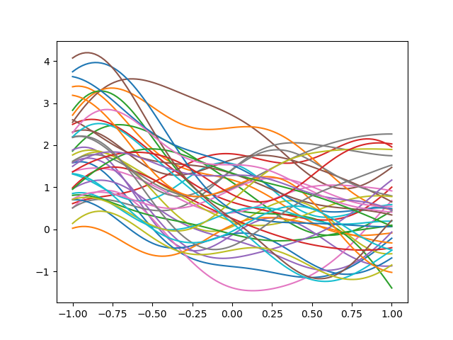
The length scale effects the variability of the GP realizations. Try chaning the length_scale to see effect on the GP realizations.

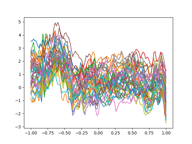
The type of kernel used by the GP also effects the GP realizations. The squared-exponential kernel above is very useful for smooth functions. For less smooth functions a Matern kernel with a smaller \(\nu\) hyper-parameter may be more effective,

other_kernel = gps.Matern(0.5, length_scale_bounds=(1e-1, 1e1), nu=0.5)
other_gp = gps.GaussianProcess(other_kernel)
for ii in range(nsamples):
    plt.plot(xx, other_gp.predict_random_realization(xx[None, :], rand_noise[:, ii:ii+1]))

Given a set of training samples \(\mathcal{Z}=\{\rv^{(m)}\}_{m=1}^M\) and associated values \(y=[y^{(1)}, \ldots, y^{(M)}]^\top\) the posterior distribution of the GP is

\[f(\cdot) \mid \theta,y \sim \mathcal{N}\left(m^\star(\cdot),C^\star(\cdot,\cdot;\theta)+\epsilon^2I\right)\]

where

\[m^\star(\rv)=t(\rv)^\top A^{-1}_\mathcal{Z}y \quad\quad C^\star(\rv,\rv^\prime)=C(\rv,\rv^\prime)-t(\rv)^\top A^{-1}_\mathcal{Z}t(\rv^\prime)\]

with

\[t(\rv)=[C(\rv,\rv^{(1)}),\ldots,C(\rv,\rv^{(N)})]^\top\]

and \(A_\mathcal{Z}\) is a matrix with with elements \((A_\mathcal{Z})_{ij}=C(\rv^{(i)},\rv^{(j)})\) for \(i,j=1,\ldots,M\). Here we dropped the dependence on the hyper-parameters \(\theta\) for convenience.

Consider the univariate Runge function

\[f(\rv) = \frac{1}{1+25\rv^2}, \quad \rv\in[-1,1]\]

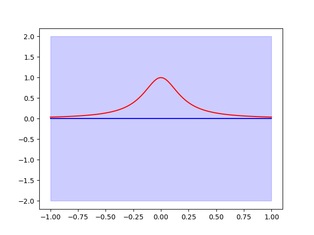
Lets construct a GP with a fixed set of training samples and associated values we can train the Gaussian process. But first lets plot the true function and prior GP mean and plus/minus 2 standard deviations using the prior covariance

def func(x):
    return 1/(1+25*x[0, :]**2)[:, np.newaxis]

validation_samples = np.linspace(lb, ub, 101)[None, :]
validation_values = func(validation_samples)
plt.plot(validation_samples[0, :], validation_values[:, 0], 'r-', label='Exact')
gp_vals, gp_std = gp(validation_samples, return_std=True)
plt.plot(validation_samples[0, :], gp_vals[:, 0], 'b-', label='GP prior mean')
_ = plt.fill_between(validation_samples[0, :], gp_vals[:, 0]-2*gp_std,
                 gp_vals[:, 0]+2*gp_std,
                 alpha=0.2, color='blue', label='GP prior uncertainty')

Now lets train the GP using a small number of evaluations and plot the posterior mean and variance.

ntrain_samples = 5
train_samples = np.linspace(lb, ub, ntrain_samples)[None, :]
train_values = func(train_samples)
gp.fit(train_samples, train_values)
print(gp.kernel_)
gp_vals, gp_std = gp(validation_samples, return_std=True)
plt.plot(validation_samples[0, :], validation_values[:, 0], 'r-', label='Exact')
plt.plot(train_samples[0, :], train_values[:, 0], 'or')
plt.plot(validation_samples[0, :], gp_vals[:, 0], '-k',
         label='GP posterior mean')
plt.fill_between(validation_samples[0, :], gp_vals[:, 0]-2*gp_std,
                 gp_vals[:, 0]+2*gp_std,
                 alpha=0.5, color='gray', label='GP posterior uncertainty')

_ = plt.legend()

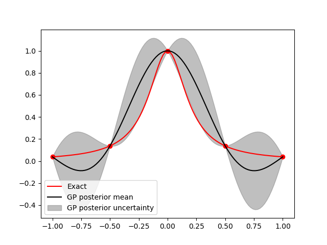
Matern(length_scale=0.441, nu=inf)

Experimental design

The nature of the training samples significantly impacts the accuracy of a Gaussian process. Noting that the variance of a GP reflects the accuracy of a Gaussian process, [SWMW1989] developed an experimental design procedure which minimizes the average variance with respect to a specified measure. This measure is typically the probability measure \(\pdf(\rv)\) of the random variables \(\rv\). Integrated variance designs, as they are often called, find a set of samples \(\mathcal{Z}\subset\Omega\subset\rvdom\) from a set of candidate samples \(\Omega\) by solving the minimization problem

\[\mathcal{Z}^\dagger=\argmin_{\mathcal{Z}\subset\Omega\subset\rvdom, \lvert\mathcal{Z}\rvert=M} \int_{\rvdom} C^\star(\rv, \rv\mid \mathcal{Z})\pdf(\rv)d\rv\]

where we have made explicit the posterior variance dependence on \(\mathcal{Z}\).

The variance of a GP is not dependent on the values of the training data, only the sample locations, and thus the procedure can be used to generate batches of samples. The IVAR criterion - also called active learning Cohn (ALC) - can be minimized over discrete [HJZ2021] or continuous [GM2016] design spaces \(\Omega\). When employing a discrete design space, greedy methods [C2006] are used to sample one at a time from a finite set of candidate samples to minimize the learning objective. This approach requires a representative candidate set which, we have found, can be generated with low-discrepancy sequences, e.g. Sobol sequences. The continuous optimization optimization is non-convex and thus requires a good initial guess to start the gradient based optimization. Greedy methods can be used to produce the initial guess, however in certain situation optimizing from the greedy design resulted in minimal improvement.

The following code plots the samples chosen by greedily minimizing the IVAR criterion

\[\int_{\rvdom} C^\star(\rv, \rv\mid \mathcal{Z})\pdf(\rv)d\rv = 1-\mathrm{Trace}\left[A_\mathcal{Z}P_\mathcal{Z}\right]\qquad P_\mathcal{Z}=\int_{\rvdom} A_{\mathcal{Z}\cup\{\rv\}}A_{\mathcal{Z}\cup\{\rv\}}^\top\pdf(\rv)d\rv\]

from a set of candidate samples \(\mathcal{Z}_\mathrm{cand}\). Because the additive constant does not effect the design IVAR designs are found by greedily adding points such that the \(N+1\) point satisfies

\[\rv_{N+1}=\argmin_{\rv^\prime\in\mathcal{Z}_\mathrm{cand}} \mathrm{Trace}\left[A_{\mathcal{Z}_N\cup\{\rv^\prime\}}P_{\mathcal{Z}_N\cup\{\rv^\prime\}}\right].\]

from pyapprox.surrogates.gaussianprocess.gaussian_process import (
    IVARSampler, GreedyIntegratedVarianceSampler, CholeskySampler)
from pyapprox.variables.joint import IndependentMarginalsVariable, stats
variable = IndependentMarginalsVariable([stats.uniform(-1, 2)])
ncandidate_samples = 101
sampler = GreedyIntegratedVarianceSampler(
    1, 100, ncandidate_samples, variable.rvs, variable,
    use_gauss_quadrature=True, econ=False,
    candidate_samples=np.linspace(
       *variable.get_statistics("interval", 1)[0, :], 101)[None, :])

kernel = gps.Matern(0.5, length_scale_bounds="fixed", nu=np.inf)
sampler.set_kernel(kernel)


def plot_gp_samples(ntrain_samples, kernel, variable):
    axs = plt.subplots(1, ntrain_samples, figsize=(ntrain_samples*8, 6))[1]
    gp = gps.GaussianProcess(kernel)
    for ii in range(1, ntrain_samples+1):
        gp.plot_1d(101, variable.get_statistics("interval", 1)[0, :], ax=axs[ii-1])

    train_samples = sampler(ntrain_samples)[0]
    train_values = func(train_samples)*0
    for ii in range(1, ntrain_samples+1):
        gp.fit(train_samples[:, :ii], train_values[:ii])
        gp.plot_1d(101, variable.get_statistics("interval", 1)[0, :], ax=axs[ii-1])
        axs[ii-1].plot(train_samples[0, :ii], train_values[:ii, 0], 'ko', ms=15)


ntrain_samples = 5
plot_gp_samples(ntrain_samples, kernel, variable)

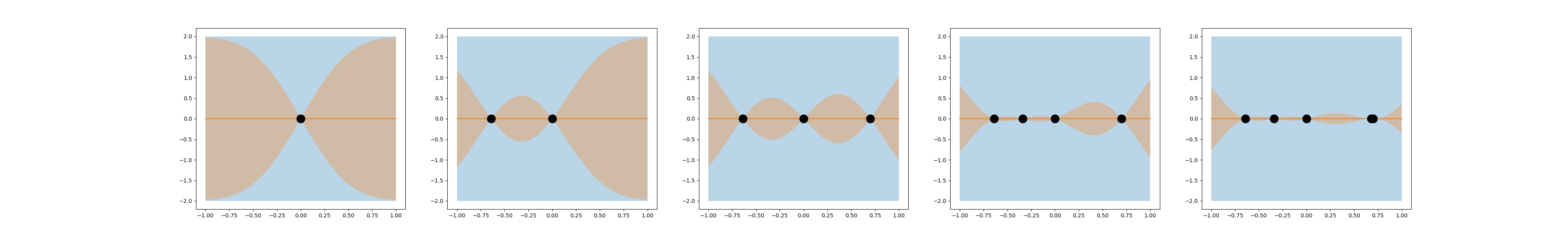
The following plots the variance obtained by a global optimiaztion of IVAR, starting from the greedy IVAR samples as the intial guess. The samples are plotted sequentially, however this is just for visualization as the global optimization does not produce a nested sequence of samples.

sampler = IVARSampler(
    1, 100, ncandidate_samples, variable.rvs, variable,
    'ivar', use_gauss_quadrature=True, nugget=1e-14)
sampler.set_kernel(kernel)
ntrain_samples = 5
plot_gp_samples(ntrain_samples, kernel, variable)

Computing IVAR designs can be computationally expensive. An alternative cheaper algorithm called active learning Mckay (ALM) greedily chooses samples that minimizes the maximum variance of the Gaussian process. That is, given M training samples the next sample is chosen via

\[\rv^{(n+1)}=\argmax_{\mathcal{Z}\subset\Omega\subset\rvdom} C^\star(\rv, \rv\mid \mathcal{Z}_M)\]

Although more computationally efficient than ALC, empirical studies suggest that ALM tends to produce GPs with worse predictive performance [GL2009].

Accurately evaluating the ALC and ALM criterion is often challenging because inverting the covariance matrix \(C(\mathcal{Z}_M\cup \rv)\) is poorly conditioned when \(\rv\) is ‘close’ to a point in \(\mathcal{Z}_M\). Consequently a small constant (nugget) is often added to the diagonal of \(C(\mathcal{Z}_M\cup \rv)\) to improve numerical stability [PW2014].

Experimental design strategies similar to ALM and ALC have been developed for radial basis functions (RBFs). The strong connections between radial basis function and Gaussian process approximation mean that the RBF algorithms can often be used for constructing GPs. A popular RBF design strategy minimizes the worst case error function (power function) of kernel based approximations [SW2006]. The minimization of the power function is equivalent to minimizing the ALM criteria [HJZ2021]. As with ALM and ALC, evaluation of the power function is unstable [SW2006]. However the authors of [PS2011] established that stability can be improved by greedily minimizing the power function using pivoted Cholesky factorization [PS2011]. Specifically, the first \(M\) pivots of the pivoted Cholesky factorization of a kernel (covariance matrix), evaluated a large set of candidate sample, define the \(M\) samples which greedily minimize the power function (ALM criteria). Minimizing the power function does not take into account any available distribution information about the inputs \(\rv\). In [HJZ2021] this information was incorporated by weighting the power function by the density \(\pdf(\rv)\) of the input variables. This procedure attempts to greedily minimizes the \(\pdf\)-weighted \(L^2\) error and produces GPs with predictive performance comparable to those based upon ALC designs while being much more computationally efficient because of its use of pivoted Cholesky factorization.

Finally we remark that while ALM and ALC are the most popular experimental design strategies for GPs, alternative methods have been proposed. Of note are those methods which approximately minimize the mutual information between the Gaussian process evaluated at the training data and the Gaussian process evaluated at the remaining candidate samples [KSG2008], [BG2016]. We do not consider these methods in our numerical comparisons.

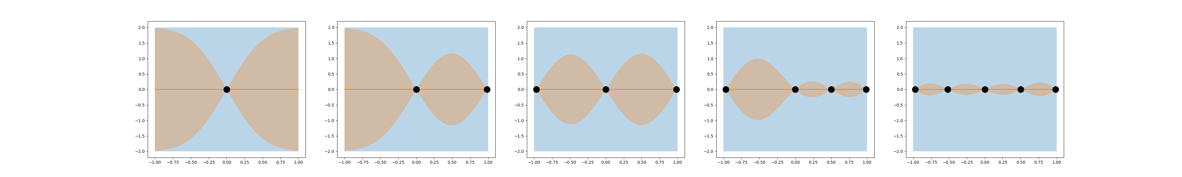
The following code shows how to use pivoted Cholesky factorization to greedily choose trainig samples for a GP.

sampler = CholeskySampler(1, 100, variable)
sampler.set_kernel(kernel)
ntrain_samples = 5
plot_gp_samples(ntrain_samples, kernel, variable)
plt.show()

Active Learning

The samples selected by the aforementioned methods depends on the kernel specified. Change the length_scale of the kernel above to see how the selected samples changes. Active learning chooses a small initial sample set then trains the GP to learn the best kernel hyper-parameters. These parameters are then used to increment the training set and then used to train the GP hyper-parameters again and so until a sufficient accuracy or computational budget is reached. PyApprox’s AdaptiveGaussianProcess implements this procedure [HJZ2021].

Constrained Gaussian processes

For certain application is it desirable for GPs to satisfy certain properties, e.g. positivity or monotonicity. See [SGFSJ2020] for a review of methods to construct constrained GPs.

References

[RW2006]

C.E. Rasmussen and C. WIlliams. Gaussian Processes for Machine Learning. MIT Press (2006)

[SWMW1989]

J. Sacks, W.J. Welch, T.J.Mitchell, H.P. Wynn Designs and analysis of computer experiments (with discussion). Statistical Science, 4:409-435 (1989)

[HJZ2021] (1,2,3,4)

H. Harbrecht, J.D. Jakeman, P. Zaspel. Cholesky-based experimental design for Gaussian process and kernel-based emulation and calibration . Communications in Computational Physics (2021) In press

[SGFSJ2020]

L.P. Swiler, M. Gulian, A. Frankel, C. Safta, J.D. Jakeman. A Survey of Constrained Gaussian Process Regression: Approaches and Implementation Challenges. Journal of Machine Learning for Modeling and Computing (2020)

[GM2016]

A. Gorodetsky, Y. Marzouk. Mercer kernels and integrated variance experimental design. Connec- tions between Gaussian process regression and polynomial approximation. SIAM/ASA J. Uncertain. Quantif., 4(1):796–828 (2016)

[C2006]

D. Cohn Neural network exploration using optimal experiment design, Neural Netw., 9 (1996), pp. 1071–1083.

[KSG2008]

A. Krause, A. Singh, C. Guestrin, Near-optimal sensor placements in Gaussian processes: Theory, efficient algorithms and empirical studies, J. Mach. Learn. Res., 9 (2008), pp. 235–284.

[PW2014]

C.Y. Peng, J. Wu, On the choice of nugget in kriging modeling for deterministic computer experiments, J. Comput. Graph. Statist., 23 (2014), pp. 151–168.

[BG2016]

J. Beck, S. Guillas, Sequential Design with Mutual Information for Computer Experiments (MICE): Emulation of a Tsunami Model, SIAM/ASA J. UNCERTAINTY QUANTIFICATION Vol. 4, pp. 739–766 (2016)

[GL2009]

R.B. Gramacy, H.K.H. Lee, Adaptive design and analysis of supercomputer experiments, Technometrics, 51 (2009), pp. 130–145.

[SW2006] (1,2)

R. Schaback and H. Wendland. Kernel techniques: From machine learning to meshless methods. Acta Numer., 15:543–639 (2006).

[PS2011] (1,2)

M. Pazouki and R. Schaback. Bases for kernel-based spaces. J. Comput. Appl. Math., 236:575–588 (2011).