Multi-index Collocation

The following provides an example of how to use multivariate quadrature, e.g. multilevel Monte Carlo, control variates to estimate the mean of a high-fidelity model from an ensemble of related models of varying cost and accuracy. Refer to Multi-level and Multi-index Collocation for a detailed tutorial on the theory behind multi-index collocation.

Load the necessary modules

from scipy import stats
import numpy as np
import matplotlib.pyplot as plt
from functools import partial
from pyapprox.benchmarks.benchmarks import setup_benchmark
from pyapprox import interface, variables, surrogates
# set seed for reproducibility
np.random.seed(1)

Set up a MultiIndexModel that takes samples \(x=[z_1,\ldots,z_D,v_1,\ldots, v_C]\) which is the concatenation of a random sample z and configuration values specifying the discretization parameters of the numerical model.

marginals = [stats.uniform(-2, 3)]
variable = variables.IndependentMarginalsVariable(marginals)


def fun(eps, zz):
    return np.cos(np.pi*(zz[0]+1)+eps)[:, None]


def setup_fun(eps):
    return partial(fun, eps)


config_values = [np.asarray([0.25, 0.125, 0])]
model = interface.MultiIndexModel(setup_fun, config_values)

Now set up and run the multi-index algorithm

config_var_trans = variables.ConfigureVariableTransformation(config_values)
mi_result = surrogates.adaptive_approximate(
    model, variable, "sparse_grid",
    {"max_nsamples": 20, "config_var_trans": config_var_trans,
     "max_level_1d": ([np.inf for ii in range(variable.num_vars())] +
                      [len(cv)-1 for cv in config_var_trans.config_values]),
     "config_variables_idx": variable.num_vars(),
     "cost_function": lambda config_sample: 2**config_sample[0],
     "tol": 1e-3, "verbose": 1})
mi_approx = mi_result.approx

Cannot add subspace [0 3]
Max level of 2 reached in variable 1
Max num evaluations (20) reached
Error estimate 0.5336307283210873
Max num evaluations (20) reached
Error estimate 0.19831215919512413
Max num evaluations (20) reached
Error estimate 0.0831164889209195

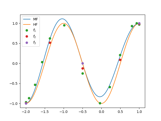
The following can be used to plot the approximation and high-fidelity target function if there is only one random variable z and one configuration variable

ax = plt.subplots()[1]
zz = np.linspace(*variable.get_statistics("interval", 1.0)[0], 101)[None, :]
ax.plot(zz[0], mi_approx(zz), label="MF")
ax.plot(zz[0], fun(0, zz), label='HF')
mi_zz_samples = mi_approx.var_trans.map_from_canonical(
    mi_approx.samples[:variable.num_vars()])
for ii in range(config_var_trans.config_values[0].shape[0]):
    II = np.where(mi_approx.samples[-1, :] == ii)[0]
    ax.plot(mi_zz_samples[0, II], mi_approx.values[II, 0], 'o',
            label=r"$f_{0}$".format(ii+1))
ax.legend()
plt.show()