Multivariate Piecewise Polynomial Interpolation

Piecewise polynomial interpolation can efficiently approximation functions with low smoothness, e.g. piecewise continuous functions. Here we will use piecewise quadratic polynomials to interpolate the discontinuous Genz benchmark. The function interpolates functions on tensor-products of 1D equidistant grids. The number of points in the grid doubles with each level. Here levels specifies the level of each 1D grid

import numpy as np
from functools import partial
from pyapprox.benchmarks import setup_benchmark
from pyapprox.analysis import visualize
from pyapprox import surrogates

benchmark = setup_benchmark("genz", test_name="discontinuous", nvars=2)

levels = [5, 5]
interp_fun = partial(
    surrogates.tensor_product_piecewise_polynomial_interpolation,
    levels=levels, fun=benchmark.fun, basis_type="quadratic")

X, Y, Z = visualize.get_meshgrid_function_data_from_variable(
    interp_fun, benchmark.variable, 50)
fig, axs = visualize.plt.subplots(1, 2, figsize=(2*8, 6))
axs[0].contourf(X, Y, Z, levels=np.linspace(Z.min(), Z.max(), 20))

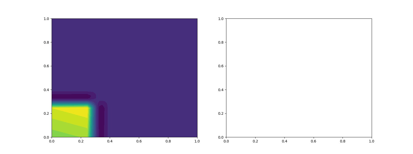
<matplotlib.contour.QuadContourSet object at 0x16ff49ff0>

To plot the difference between the interpolant and the target function use

X, Y, Z = visualize.get_meshgrid_function_data_from_variable(
    lambda x: interp_fun(x)-benchmark.fun(x), benchmark.variable, 50)
axs[1].contourf(X, Y, Z, levels=np.linspace(Z.min(), Z.max(), 20))
visualize.plt.show()