Low-discrepancy quadrature

Monte Carlo

It is often important to quantify statistics of numerical models. Monte Carlo quadrature is the simplest and most robust method for doing so. For any model we can compute statistics, such as mean and variance as follows

from pyapprox import expdesign
from pyapprox.benchmarks import setup_benchmark
benchmark = setup_benchmark("genz", test_name="oscillatory", nvars=2)
nsamples = 100
mc_samples = benchmark.variable.rvs(nsamples)
values = benchmark.fun(mc_samples)
mean = values.mean(axis=0)
variance = values.var(axis=0)
print("mean", mean)
print("variance", variance)

mean [-0.49820729]
variance [0.03984726]

Although not necessary for this scalar valued function, we in geenral must use the args axis=0 to mean and variance so that we compute the statistics for each quantity of interest (column of values)

Sobol Sequences

Large number of samples are needed to compute statistics using Monte Carlo quadrature. Low-discrepancy sequences can be used to improve accuracy for a fixed number of samples. We can compute statistics using Sobol sequences as follows

sobol_samples = expdesign.sobol_sequence(
    benchmark.variable.num_vars(), nsamples, variable=benchmark.variable)
values = benchmark.fun(sobol_samples)
from pyapprox.variables import print_statistics
print_statistics(sobol_samples, values)

           z0         z1         y0
count  100.000000 100.000000 100.000000
mean     0.494063   0.497812  -0.464285
std      0.288799   0.288344   0.198696
min      0.000000   0.000000  -0.837224
max      0.992188   0.992188   0.000000

Here we have used print statistics to compute the sample stats. Note, the inverse cumulative distribution functions of the univariate variables in variable are used to ensure that the samples integrate with respect to the joint distribution of variable. If the variable argument is not provided the Sobol sequence will be generated on the unit hybercube \([0,1]^D\).

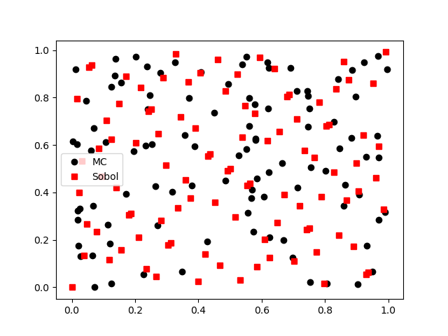
Low-discrepancy sequences are typically more evenly space over the parameter space. This can be seen by comparing the Monte Carlo and Sobol sequence samples

import matplotlib.pyplot as plt
plt.plot(mc_samples[0, :], mc_samples[1, :], 'ko', label="MC")
plt.plot(sobol_samples[0, :], sobol_samples[1, :], 'rs', label="Sobol")
plt.legend()
plt.show()

#
#Halton Sequences
#================
#Pyapprox also supports Halton Sequences
halton_samples = expdesign.halton_sequence(
    benchmark.variable.num_vars(), nsamples, variable=benchmark.variable)
values = benchmark.fun(halton_samples)
print_statistics(halton_samples, values)

           z0         z1         y0
count  100.000000 100.000000 100.000000
mean     0.488438   0.484856  -0.454770
std      0.288831   0.290073   0.199483
min      0.000000   0.000000  -0.803806
max      0.984375   0.987654   0.000000

Latin Hypercube Designs

Latin Hypercube designs are another popular means to compute low-discrepancy samples for quadrature. Pyapprox does not support such designs as unlike Sobol and Halton Sequences they are not nested. For example, when using Latin Hypercube designs, it is not possible to requrest 100 samples then request 200 samples while resuing the first 100.