Multivariate Lagrange Interpolation

For smooth function Lagrange polynomials can be used to interpolate univariate functions evaluated on a tensor-product grid. Pyapprox uses the Barycentric formulation of Lagrange interpolation which is more efficient and stable than traditional Lagrange interpolation.

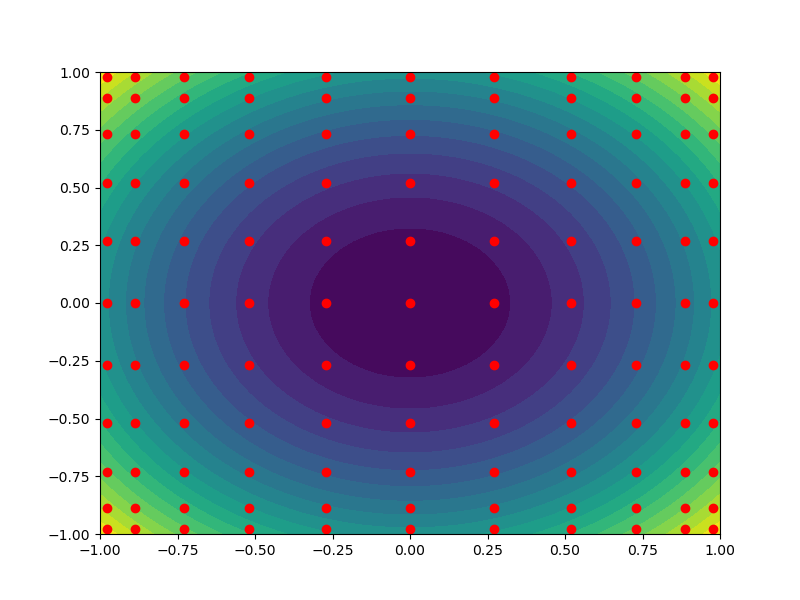
We must define the univariate grids that we will use to construct the tensor product grid. While technically Lagrange interpolation can be used with any 1D grids, it is better to use points well suited to polynomial interpolation. Here we use the samples of a Gaussian quadrature rule.

from scipy import stats
import numpy as np
import matplotlib.pyplot as plt
from functools import partial
from pyapprox import surrogates
from pyapprox.analysis import visualize
from pyapprox import variables
from pyapprox import util

degree = 10
marginals = [stats.uniform(-1, 2), stats.uniform(-1, 2)]
grid_samples_1d = [surrogates.get_gauss_quadrature_rule_from_marginal(
    rv, degree+1)(degree+1)[0] for rv in marginals]

Now lets define the function we want to interpolate, e.g. \(f(\rv)=\rv_1^2+\rv_2^2\)

def fun(samples):
    return np.sum(samples**2, axis=0)[:, None]


##%
#Now we will use partial to create a callable function that just takes
#the samples at which we want to evaluate the interpolant
#This function will evaluate fun on a tensor product grid internally
interp_fun = partial(
    surrogates.tensor_product_barycentric_lagrange_interpolation,
    grid_samples_1d, fun)
variable = variables.IndependentMarginalsVariable(marginals)
X, Y, Z = visualize.get_meshgrid_function_data_from_variable(
    interp_fun, variable, 50)
fig, ax = plt.subplots(1, 1, figsize=(8, 6))
ax.contourf(X, Y, Z, levels=np.linspace(Z.min(), Z.max(), 20))
util.plot_2d_samples(
    util.cartesian_product(grid_samples_1d), ax, marker='o', c='r')
plt.show()

Barycentric interpolation can be used for any number of variables. However, the number of evaluations of the target function grows exponentially with the number of variables