Random Variables

This tutorial describes how to create multivariate random variable objects.

PyApprox supports multivariate random variables comprised of independent univariate variables. Such variables can be defined from a list of scipy.stats variable objects. To create a Beta random variable defined on \([0, 1]\times[1, 2]\)

from pyapprox.variables import IndependentMarginalsVariable
from scipy import stats
marginals = [stats.beta(2, 3, loc=0, scale=1),
             stats.beta(5, 2, loc=1, scale=1)]
variable = IndependentMarginalsVariable(marginals)

A summary of the random variable can be printed using

print(variable)

Independent Marginal Variable
Number of variables: 2
Unique variables and global id:
    beta(a=2,b=3,loc=[0],scale=[1]): z0
    beta(a=5,b=2,loc=[1],scale=[1]): z1

To generate random samples from the multivariate variable use

nsamples = 10
samples = variable.rvs(nsamples)

For such 2D variables comprised of continuous univariate random variables we can evaluate the joint probability density function (PDF) at a set of samples using

pdf_vals = variable.pdf(samples)
print(pdf_vals)

[[1.61857392]
 [1.95802036]
 [0.60604613]
 [2.46081611]
 [2.19411368]
 [2.8227188 ]
 [3.43022837]
 [3.25501853]
 [3.0926788 ]
 [3.29308097]]

Any statistics, supported by the univariate scipy.stats variables, can be accessed for all 1D variabels using pyapprox.variables.IndependentMarginalsVariable.get_statistics() For example,

mean = variable.get_statistics("mean")
variance = variable.get_statistics("var")
print("Mean", mean)
print("Variance", variance)

Mean [[0.4       ]
 [1.71428571]]
Variance [[0.04     ]
 [0.0255102]]

Note, by convention PyApprox tries to always return 2D numpy arrays, e.g. here we are returning a column vector. Sometimes this is not possible because some functions in other packages, such as SciPy, require input as 1D arrays.

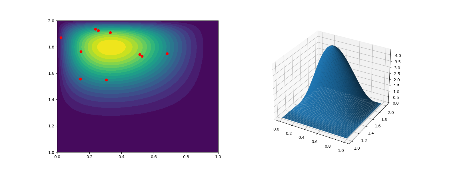
We can also plot the joint PDF and overlay the random samples. Given a number of 1D samples specified by the user, the following plots evaluates the PDF (or any 2D function) on a cartesian grid of these 1D samples defined on the bounded ranges of the random variables. If some univariate variables are unbounded then the range corresponding to a fraction of the total probability will be used. See the documentation at pyapprox.util.visualization.get_meshgrid_function_data_from_variable()

from pyapprox.analysis.visualize import (
    get_meshgrid_function_data_from_variable)
nplot_pts_1d = 50
X, Y, Z = get_meshgrid_function_data_from_variable(
    variable.pdf, variable, nplot_pts_1d)

Here we will create 2D subplots, a contour plot and a surface plot

import matplotlib.pyplot as plt
import numpy as np
ncontours = 20
fig = plt.figure(figsize=(2*8, 6))
ax0 = fig.add_subplot(1, 2, 1)
ax0.plot(samples[0, :], samples[1, :], 'ro')
ax0.contourf(
    X, Y, Z, levels=np.linspace(Z.min(), Z.max(), ncontours))
ax1 = fig.add_subplot(1, 2, 2, projection='3d')
ax1.plot_surface(X, Y, Z)
plt.show()

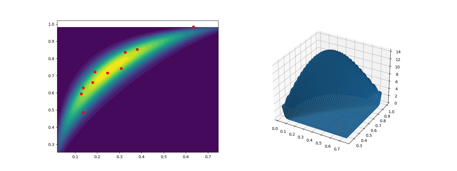
We can also generate samples using Gaussian copulas. First specify the

marginals and the correlation between them

from pyapprox.variables import GaussCopulaVariable
marginals = [stats.beta(a=2, b=5), stats.beta(a=5, b=2)]
x_correlation = np.array([[1, 0.9], [0.9, 1]])
variable = GaussCopulaVariable(marginals, x_correlation)

samples = variable.rvs(nsamples)
nplot_pts_1d = 50
X, Y, Z = get_meshgrid_function_data_from_variable(
    variable.pdf, variable, nplot_pts_1d)
ncontours = 20
fig = plt.figure(figsize=(2*8, 6))
ax0 = fig.add_subplot(1, 2, 1)
ax0.plot(samples[0, :], samples[1, :], 'ro')
ax0.contourf(
    X, Y, Z, levels=np.linspace(Z.min(), Z.max(), ncontours))
ax1 = fig.add_subplot(1, 2, 2, projection='3d')
ax1.plot_surface(X, Y, Z)
plt.show()