Parameter Sweeps

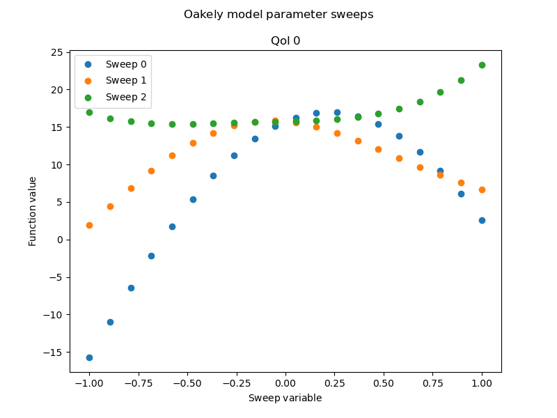
When analyzing complex models or functions it is often useful to gain insight into its smoothness and non-linearity before undertaking more computationally intensive analysis such as uncertainty quantification or sensitivity analysis. Knowledge about smoothness and non-linearity can be used to inform what algorithms are used for these later tasks.

Lets first generate parameter sweeps for the oakley benchmark. Each sweep will be a random direction through the parameter domain. The domain is assumed to be the cartesian product of the centered truncated intervals of each 1D variable marginal. For unbounded variables each interval captures 99% of the PDF. For bounded variables the true bounds are used (i.e. are not truncated)

from pyapprox import analysis
from pyapprox.util.visualization import plt, mathrm_label
from pyapprox.benchmarks import setup_benchmark
import numpy as np
np.random.seed(1)

benchmark = setup_benchmark("oakley")
axs = analysis.generate_parameter_sweeps_and_plot_from_variable(
    benchmark.fun, benchmark.variable, num_samples_per_sweep=20, num_sweeps=3)
plt.gcf().suptitle(mathrm_label("Oakely model parameter sweeps"))
plt.show()

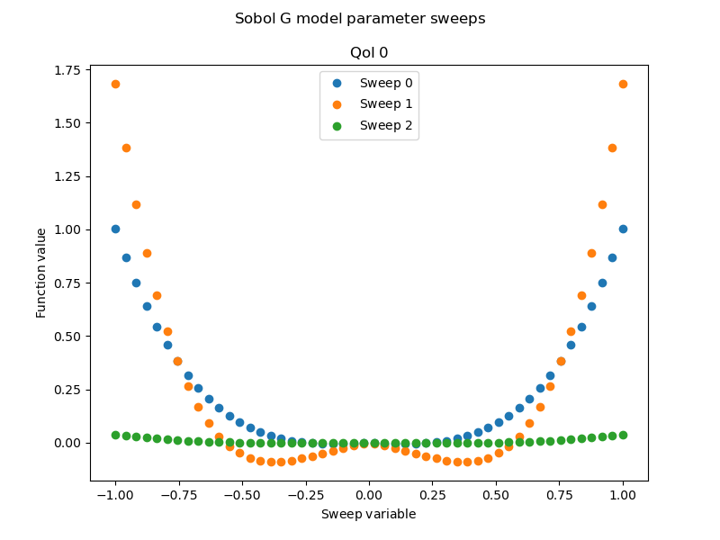
Now lets plot parameter sweeps for the Sobol G function

benchmark = setup_benchmark("sobol_g", nvars=4)
axs = analysis.generate_parameter_sweeps_and_plot_from_variable(
    benchmark.fun, benchmark.variable, num_samples_per_sweep=50, num_sweeps=3)
plt.gcf().suptitle(mathrm_label("Sobol G model parameter sweeps"))
plt.show()

[2.10729798e-04 2.16355425e-01 4.96284418e-04 4.46077822e-05] [0.99978927 0.78364457 0.99950372 0.99995539]

The Sobol G function is not as smooth as the Oakely function. The former has discontinuous first derivatives which can be seen by inspecting their aprameter sweeps