Univariate Gaussian Quadrature

Univariate Gaussian quadrature can be used to efficiently integrate smooth one-dimensional functions. While numpy supports Hermite and Legendre Gaussian qurature, Pyapprox can generate Gaussian quadrature rules for any continouous random variable implemented in scipy.stats.

To generate a univariate quadrature rule for uniform random variables

from pyapprox import surrogates
from scipy import stats
degree = 10

scipy_var = stats.uniform(-1, 2)
quad_rule = surrogates.get_gauss_quadrature_rule_from_marginal(
    scipy_var, degree+1)
x_quad, w_quad = quad_rule(5)

As an example, we can use this quadrature rule to integrate \(\rv^2\) with repsect to the uniform PDF on [-1, 1], i.e. 1/2

values = x_quad**2
integral = values.dot(w_quad)
print(integral)

0.3333333333333332

The quadrature recovers the integral value of 1/3 to machine precision. Note unlike leggauss we are integrating with resepect to the uniform PDF.

The function is also capable of generating rules on different intervals For example

scipy_var = stats.uniform(0, 2)
x_quad, w_quad = surrogates.get_gauss_quadrature_rule_from_marginal(
    scipy_var, degree+1)(degree)
values = x_quad**2
integral = values.dot(w_quad)
print(integral)

1.3333333333333346

Quadrature rules can be created for almost any random variable. Here we will generate a quadrature rule for an exponential random variable

scipy_var = stats.expon()
x_quad, w_quad = surrogates.get_gauss_quadrature_rule_from_marginal(
    scipy_var, degree+1)(degree)
values = x_quad**2
integral = values.dot(w_quad)
print(integral)

2.000000000000001

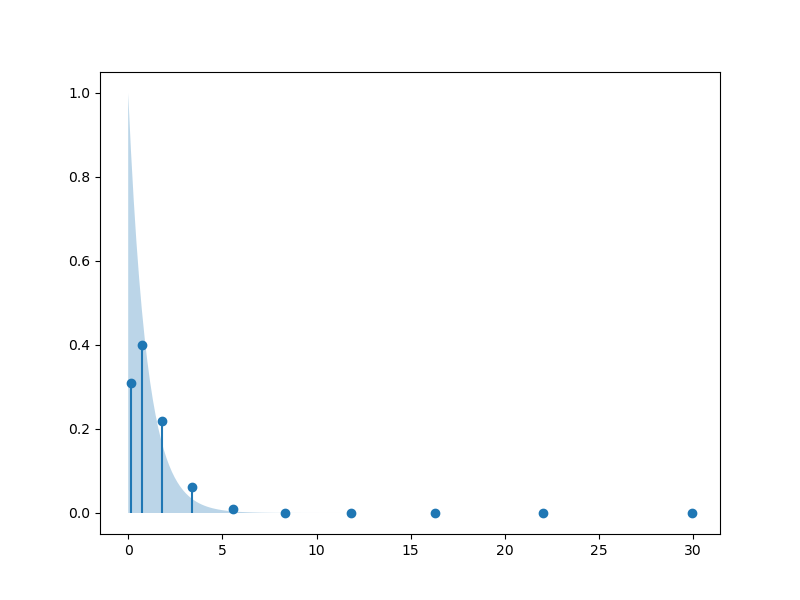
For interest, we plot the quadrature rule against the PDF of the exponential variable

import numpy as np
import matplotlib.pyplot as plt
from pyapprox.analysis import visualize
from pyapprox.variables import marginals
visualize.plot_discrete_measure_1d(x_quad, w_quad)
vrange = marginals.get_truncated_range(scipy_var, 1-1e-6)
xx = np.linspace(vrange[0], vrange[1], 101)
plt.fill_between(xx, 0*xx, scipy_var.pdf(xx), alpha=0.3)
plt.show()