Note
Go to the end to download the full example code
End-to-End Model Analysis
This tutorial describes how to use each of the major model analyses in Pyapprox following the exposition in [PYAPPROX2023].
First lets load all the necessary modules and set the random seeds for reproducibility.
from scipy import stats
import numpy as np
import matplotlib as mpl
import matplotlib.pyplot as plt
from functools import partial
import torch
import time
from pyapprox.util.visualization import mathrm_label
from pyapprox.variables import (
    IndependentMarginalsVariable, print_statistics, AffineTransform)
from pyapprox.benchmarks import setup_benchmark, list_benchmarks
from pyapprox.interface.wrappers import (
    TimerModel, WorkTrackingModel,
    evaluate_1darray_function_on_2d_array)
from pyapprox.surrogates import adaptive_approximate
from pyapprox.analysis.sensitivity_analysis import (
    run_sensitivity_analysis, plot_sensitivity_indices)
from pyapprox.bayes.metropolis import (
    loglike_from_negloglike, plot_unnormalized_2d_marginals)
from pyapprox.bayes.metropolis import MetropolisMCMCVariable
from pyapprox.expdesign.bayesian_oed import get_bayesian_oed_optimizer
from pyapprox import multifidelity
# import warnings
# warnings.filterwarnings("ignore", category=DeprecationWarning)
np.random.seed(2023)
_ = torch.manual_seed(2023)
The tutorial can save the figures to file if desired. If you do want the plots set savefig=True
# savefig = True
savefig = False
The following code shows how to create and sample from two independent uniform random variables defined on \([-2, 2]\). We use uniform variables here, but any marginal from the scipy.stats module can be used.
nsamples = 30
univariate_variables = [stats.uniform(-2, 4), stats.uniform(-2, 4)]
variable = IndependentMarginalsVariable(univariate_variables)
samples = variable.rvs(nsamples)
print_statistics(samples)
           z0         z1
count   30.000000  30.000000
mean    -0.528053   0.197078
std      0.905072   1.114676
min     -1.911641  -1.684959
max      1.722128   1.922229
PyApprox supports various types of variable transformations. The following code shows how to use an affinte transformation to map samples from variables to samples from the variable’s canonical form.
var_trans = AffineTransform(variable)
canonical_samples = var_trans.map_to_canonical(samples)
print_statistics(canonical_samples)
           z0         z1
count   30.000000  30.000000
mean    -0.264027   0.098539
std      0.452536   0.557338
min     -0.955821  -0.842480
max      0.861064   0.961114
Pyapprox provides many utilities for interfacing with complex numerical codes. The following shows how to wrap a model and store the wall time required to evaluate each sample in a set. First define a function with a random execution time that takes in one sample at a time, i.e. a 1D array. Then wrap that model so that multiple samples can be evaluated at once.
def fun_pause_1(sample):
    assert sample.ndim == 1
    time.sleep(np.random.uniform(0, .05))
    return np.sum(sample**2)


def pyapprox_fun_1(samples):
    return evaluate_1darray_function_on_2d_array(fun_pause_1, samples)
Now wrap the latter function and run it while tracking their execution times. The last print statement prints the median execution time of the model.
timer_model = TimerModel(pyapprox_fun_1)
model = WorkTrackingModel(timer_model)
values = model(samples)
print(model.work_tracker())
[0.02981555]
Other wrappers available in PyApprox include those for running multiple models at once, useful for multi-fidelity methods, wrappers that fix a subset of inputs to user specified values, wrappers that only return a subset of all possible model ouputs, and wrappers for evaluating samples in parallel.
Pyapprox provide numerous benchmarks for verifying, validating and comparing model analysis algorithms. The following list the names of all benchmarks and then creates a benchmark that can be used to test the creation of surrogates, Bayesian inference, and optimal experimental design. This benchmark requires determining the true coefficients of the Karhunene Loeve expansion (KLE) used to characterize the uncertain diffusivity field of an advection diffusion equation. See documentation of the benchmark for more details).
print(list_benchmarks())
noise_stdev = 1  # 1e-1
inv_benchmark = setup_benchmark(
    "advection_diffusion_kle_inversion", kle_nvars=3,
    noise_stdev=noise_stdev, nobs=5, kle_length_scale=0.5)
print(inv_benchmark)
['sobol_g', 'ishigami', 'oakley', 'rosenbrock', 'genz', 'cantilever_beam', 'wing_weight', 'piston', 'chemical_reaction', 'random_oscillator', 'coupled_springs', 'hastings_ecology', 'multi_index_advection_diffusion', 'advection_diffusion_kle_inversion', 'polynomial_ensemble', 'tunable_model_ensemble', 'multioutput_model_ensemble', 'short_column_ensemble', 'parameterized_nonlinear_model']
Benchmark(negloglike, variable, noiseless_obs, obs, true_sample, obs_indices, obs_fun, KLE, mesh)
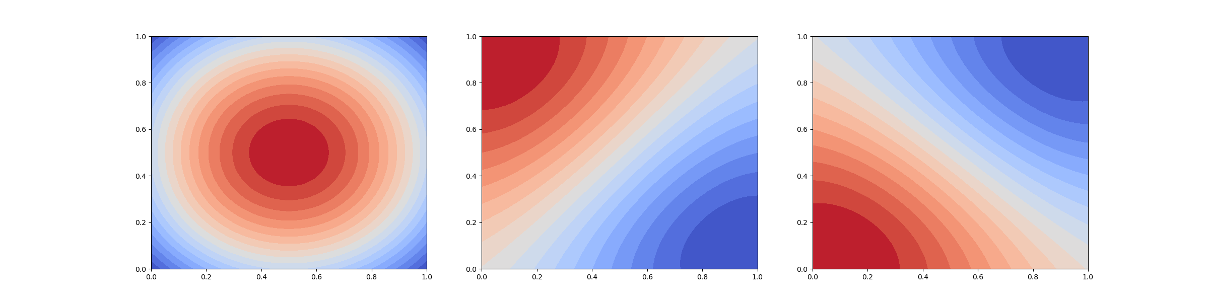
The following plots the modes of the KLE
fig, axs = plt.subplots(
    1, inv_benchmark.KLE.nterms, figsize=(8*inv_benchmark.KLE.nterms, 6))
for ii in range(inv_benchmark.KLE.nterms):
    inv_benchmark.mesh.plot(inv_benchmark.KLE.eig_vecs[:, ii:ii+1], 50,
                            ax=axs[ii])
PyApprox provides many popular methods for constructing surrogates that once constructed can be evaluated in place of a computaionally expensive simulation model in model analyses. The following code creates a Gaussian process (GP) surrogate. The function used to construct the surrogate takes a callback which is evaluated each time the adaptive surrogate is refined. Here we use to compute the error of the surrogate as it is constructed using validation data. Uncomment the code to use a polynomial based surrogate instead of a GP. The user does not have to change any subsequent code
validation_samples = inv_benchmark.variable.rvs(100)
validation_values = inv_benchmark.negloglike(validation_samples)
nsamples, errors = [], []
def callback(approx):
    nsamples.append(approx.num_training_samples())
    error = np.linalg.norm(
        approx(validation_samples)-validation_values, axis=0)
    error /= np.linalg.norm(validation_values, axis=0)
    errors.append(error)

approx_result = adaptive_approximate(
    inv_benchmark.negloglike, inv_benchmark.variable, "gaussian_process",
    {"max_nsamples": 50, "ncandidate_samples": 2e3, "verbose": 0,
     "callback": callback, "kernel_variance": 400})

# approx_result = adaptive_approximate(
#     inv_benchmark.negloglike, inv_benchmark.variable, "polynomial_chaos",
#     {"method": "leja", "options": {
#         "max_nsamples": 100, "ncandidate_samples": 3e3, "verbose": 0,
#         "callback": callback}})
approx = approx_result.approx
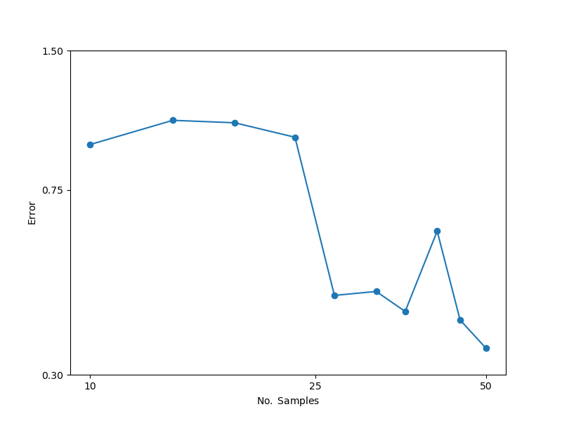
We can plot the errors obtained from the callback with
ax = plt.subplots(figsize=(8, 6))[1]
ax.loglog(nsamples, errors, "o-")
ax.set_xlabel(mathrm_label("No. Samples"))
ax.set_ylabel(mathrm_label("Error"))
ax.set_xticks([10, 25, 50])
ax.set_yticks([0.3, 0.75, 1.5])
ax.get_xaxis().set_major_formatter(mpl.ticker.ScalarFormatter())
ax.minorticks_off()
ax.get_yaxis().set_major_formatter(mpl.ticker.ScalarFormatter())
#ax.tick_params(axis='y', which='minor', bottom=False)
if savefig:
    plt.savefig("gp-error-plot.pdf")
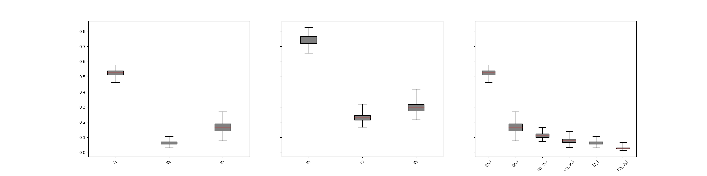
Now we will perform a sensitivity analysis. Specifically we compute variance based sensitivity indices that measure the impact of each KLE mode on the mismatch between the observed data and the model predictions. We use the negative log likelihood to characterize this mismatch. Here we have used the surrogate to speed up the computation of the sensitivity indices. Uncomment the commented code to use the numerical model. Note the drastic increase in computational cost. Warning: using the numerical model will take many minutes. The plots in the figure, generated from left to right are: main effect, largest Sobol indices and total effect indices.
sa_result = run_sensitivity_analysis(
    "surrogate_sobol", approx, inv_benchmark.variable)
# sa_result = run_sensitivity_analysis(
#     "sobol", benchmark.negloglike, inv_benchmark.variable)
axs = plot_sensitivity_indices(
    sa_result)[1]
if savefig:
    plt.savefig("gp-sa-indices.pdf", bbox_inches="tight")
Now we will use the surrogate with Bayesian inference to learn the coefficients of the KL. Specifically we will draw a set of samples from the posterior distribution of the KLE given the observed data provided in the benchmark.
But First we will improve the accuracy of the surrogate and print out the error which can be compared to the errors previously plotted. The error of the original surrogate was kept low to demonstrate the ability to quantify error in the sensitivity indices from using a surrogate.
approx.refine(100)
error = np.linalg.norm(
    approx(validation_samples)-validation_values, axis=0)
error /= np.linalg.norm(validation_values, axis=0)
print("Surrogate", error)
Surrogate [0.06476258]
Now create a MCMCVariable to sample from the posterior. The benchmark has already formulated the negative log likelihood that is needed. Here we will use PyApprox’s native delayed rejection adaptive metropolis (DRAM) sampler.
Uncomment the commented code to use the numerical model instead of the surrogate with the MCMC algorithm. Again note the significant increase in computational time
npost_samples = 200
loglike = partial(loglike_from_negloglike, approx)
# loglike = partial(loglike_from_negloglike, inv_benchmark.negloglike)
mcmc_variable = MetropolisMCMCVariable(
    inv_benchmark.variable, loglike, method_opts={"cov_scaling": 1})
print(mcmc_variable)
map_sample = mcmc_variable.maximum_aposteriori_point()
print("Computed Map Point", map_sample[:, 0])
post_samples = mcmc_variable.rvs(npost_samples)
print("Acceptance rate", mcmc_variable._acceptance_rate)
JointVariable
Computed Map Point [0.28587284 0.73868579 0.99888313]
Acceptance rate 0.43
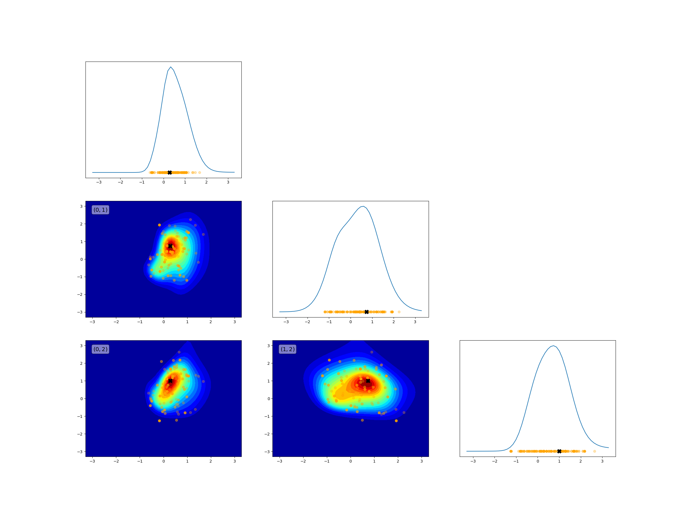
Now plot the posterior samples with the 2D Marginals of the posterior. Note do not do this with the numerical model as this would take an eternity due to the cost of evaluating the numerical model, which is much higher relative to the cost of running the surrogate.
plot_unnormalized_2d_marginals(
    mcmc_variable._variable, mcmc_variable._loglike, nsamples_1d=50,
    plot_samples=[
        [post_samples, {"alpha": 0.3, "c": "orange"}],
        [map_sample, {"c": "k", "marker": "X", "s": 100}]],
    unbounded_alpha=0.999)
if savefig:
    plt.savefig("posterior-samples.pdf", bbox_inches="tight")
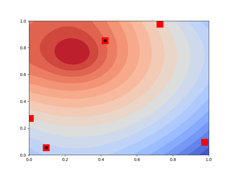
In the Bayesian inference above we used a fixed number of observations at randomly chosen spatial locations. However choosing observation locations is usually a poor idea. Not all observations can reduce the uncertainty in the parameters equally. Here we use Bayesian optimal experimental design to choose the 3 best design locations from the previously observed 10 pretending that we do not know the value of the observations.
fig, ax = plt.subplots(1, 1, figsize=(8, 6))
#plot a single solution to the PDE before overlaying the designs
inv_benchmark.mesh.plot(
    inv_benchmark.obs_fun._fwd_solver.solve()[:, None], 50, ax=ax)

ndesign = 3
design_candidates = inv_benchmark.mesh.mesh_pts[:, inv_benchmark.obs_indices]
ndesign_candidates = design_candidates.shape[1]
oed = get_bayesian_oed_optimizer(
    "kl_params", ndesign_candidates, inv_benchmark.obs_fun, noise_stdev,
    inv_benchmark.variable, max_ncollected_obs=ndesign)
oed_results = []
for step in range(ndesign):
    results_step = oed.update_design()[1]
    oed_results.append(results_step)
selected_candidates = design_candidates[:, np.hstack(oed_results)]
print(selected_candidates)
ax.plot(design_candidates[0, :], design_candidates[1, :], "rs", ms=16)
ax.plot(selected_candidates[0, :], selected_candidates[1, :], "ko")
if savefig:
    plt.savefig("oed-selected-design.pdf")
Running 1000 outer model evaluations
Predicted observation bounds 14.477297168295355 1.1388690449350853
Evaluations took 12.507869958877563
Running 1000 inner model evaluations
Evaluations took 12.18462586402893
Computing utilities in serial took 0.2077329158782959
Computing utilities in serial took 0.023710250854492188
Computing utilities in serial took 0.03223991394042969
[[0.0954915  0.42178277 0.42178277]
 [0.05449674 0.85355339 0.85355339]]
Note that typically optimal experimental design (OED) would be used before conducting Bayesian inference. However, because understanding of Bayesian inference is needed to understand Bayesian OED we reversed the order. OED is much more expensive than a single Bayesian calibration because it requires solving many calibration problems. So typically we do not solve the calibration problems in the OED procedure to the same degree of accuracy as a final calibration. The accuracy of the calibrations used by OED must only be sufficient to distinguish between designs. This accuracy is typically much lower than the accuracy required in estimates of uncertainty in the parameters or predictions needed for decision making tasks such as risk assessment.
Here we will set up a related benchmark to the one we have been using, which can be used to demonstrate the forward propagation of uncertainty. This benchmark uses the steady state solution of the advection diffusion, obtained with a constant addition of a tracer into the domain at a single source model as initial condition. A pump at another locations is then activated to extract the tracer from the domain. The benchmark quantity of interest measures the change of the tracer concentration in a subomain. The benchmark provides models of varying cost and accuracy that use different discretizations of the spatial PDE mesh and number of time steps which can be used with multi-fideilty methods. To setup the benchmark use the following
fwd_benchmark = setup_benchmark(
    "multi_index_advection_diffusion",
    kle_nvars=inv_benchmark.variable.num_vars(), kle_length_scale=0.5,
    time_scenario=True)
model = WorkTrackingModel(
    TimerModel(fwd_benchmark.model_ensemble), num_config_vars=1)
Here we will use Multi-fidelity statistical estimation to compute the mean value of the QoI to account for the uncertainty in the KLE cofficients. So first we must compute the covariance between the QoI returned by each of our models. We use samples from the posterior. But uncommenting the code below will use samples from the prior.
npilot_samples = 20
generate_samples = inv_benchmark.variable.rvs  # for sampling from prior
# generate_samples = post_samples
cov = multifidelity.estimate_model_ensemble_covariance(
    npilot_samples, generate_samples, model,
    fwd_benchmark.model_ensemble.nmodels)[0]
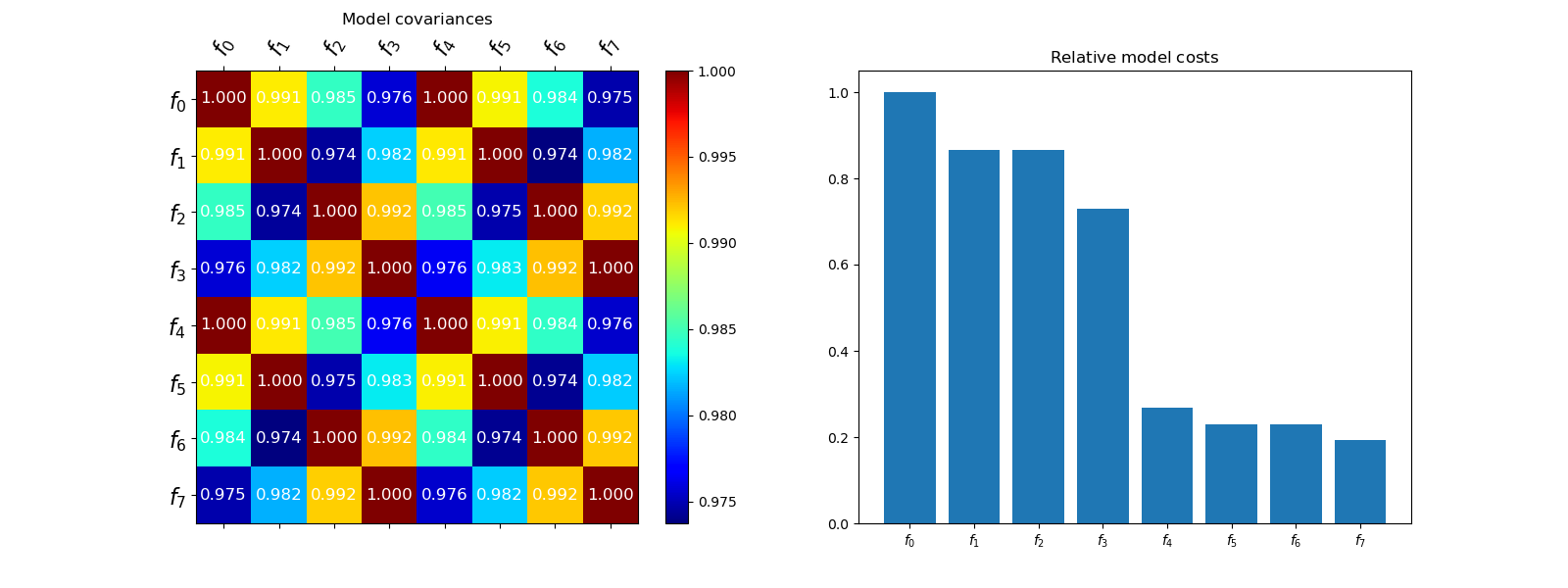
By using a WorkTrackingModel we can extract the median costs of evaluatin each model which is needed to predict the error of the multi-fidelity estimate of the mean which we can compare to a prediction of the single fidelity estimate that only uses the highest fidelity model.
model_ids = np.asarray([np.arange(fwd_benchmark.model_ensemble.nmodels)])
model_costs = model.work_tracker(model_ids)
# make costs in terms of fraction of cost of high-fidelity evaluation
model_costs /= model_costs[0]
Now visualize the correlation between the models and their computational cost relative to the highest-fidelity model cost
fig, axs = plt.subplots(1, 2, figsize=(2*8, 6))
multifidelity.plot_correlation_matrix(
    multifidelity.get_correlation_from_covariance(cov), ax=axs[0])
multifidelity.plot_model_costs(model_costs, ax=axs[1])
axs[0].set_title(mathrm_label("Model covariances"))
_ = axs[1].set_title(mathrm_label("Relative model costs"))
Now find the best multi-fidelity estimator among all available options Note, the exact predicted variance will change from run to run even with the same seed because the computational time measured will change slightly for each run
stat = multifidelity.multioutput_stats["mean"](1)
stat.set_pilot_quantities(cov)

best_est = multifidelity.get_estimator(
    "gmf", stat, model_costs, tree_depth=4, allow_failures=True,
    max_nmodels=4)

target_cost = 1e2
best_est.allocate_samples(target_cost)
print("Predicted variance",
      best_est._covariance_from_npartition_samples(
          best_est._rounded_npartition_samples))
Predicted variance tensor([[7.5268e-06]])
Now we can plot the relative performance of the single and multi-fidelity estimates of the mean before requiring any additional model evaluations
fig, axs = plt.subplots(1, 2, figsize=(2*8, 6))
multifidelity.plot_estimator_variance_reductions([best_est], ["Best"], axs[0])
model_labels = [
    r"$f_{%d}$" % ii for ii in np.arange(fwd_benchmark.model_ensemble.nmodels)]
multifidelity.plot_estimator_sample_allocation_comparison(
    [best_est], model_labels, axs[1])
if savefig:
    plt.savefig("acv-variance-reduction.pdf")
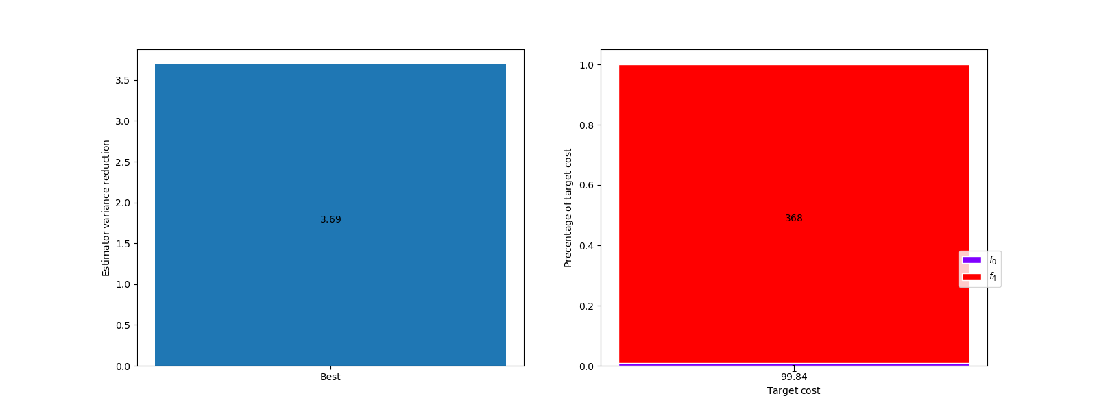
It is clear that the multi-fidelity estimator will be more computationally efficient. Once the user is ready to actually estimate the mean QoI they can use
print(fwd_benchmark)
samples_per_model = best_est.generate_samples_per_model(
    fwd_benchmark.variable.rvs)
best_models = [fwd_benchmark.model_ensemble.functions[idx] for
               idx in best_est._best_model_indices]
values_per_model = [
    fun(samples) for fun, samples in zip(best_models, samples_per_model)]
mean = best_est(values_per_model)
print("Mean QoI", mean)

plt.show()
Benchmark(fun, variable, get_num_degrees_of_freedom, config_var_trans, model_ensemble, funs)
Mean QoI [0.50175498]
References
Total running time of the script: ( 2 minutes 10.042 seconds)