Generalized Approximate Control Variate Monte Carlo

This tutorial builds upon Approximate Control Variate Monte Carlo, Multi-level Monte Carlo, and Multi-fidelity Monte Carlo. MLMC and MFMC are two approaches which can utilize an esemble of models of vary cost and accuracy to efficiently estimate the expectation of the highest fidelity model. In this tutorial we introduce a general framework for ACVMC when using 2 or more mmodels. We show that MFMC are both instances of this framework and use the flexibility of the framework to derive new ACV estimators.

Control variate Monte Carlo can be easily extended and applied to more than two models. Consider \(M\) lower fidelity models with sample ratios \(r_\alpha>=1\), for \(\alpha=1,\ldots,M\). The approximate control variate estimator of the mean of the high-fidelity model \(Q_0=\mean{f_0}\) is

\[\begin{split}Q^{\text{ACV}} &= Q_{0,\mathcal{Z}_{0,1}} + \sum_{\alpha=1}^M \eta_\alpha \left( Q_{\alpha,\mathcal{Z}_{\alpha,1}} - \mu_{\alpha,\mathcal{Z}_{\alpha,2}} \right) =Q_{0,\mathcal{Z}_{0,1}} + \sum_{\alpha=1}^M \eta_\alpha \Delta_{\alpha,\mathcal{Z}_{\alpha,1},\mathcal{Z}_{\alpha,2}}\\&=Q_{0,N}+\V{\eta}\V{\Delta}\end{split}\]

Here \(\V{\eta}=[\eta_1,\ldots,\eta_M]^T\), \(\V{\Delta}=[\Delta_1,\ldots,\Delta_M]^T\), and \(\mathcal{Z}_{\alpha,1}\), \(\mathcal{Z}_{\alpha,2}\) are sample sets that may or may not be disjoint. Specifying the exact nature of these sets, including their cardinality, can be used to design different ACV estimators which will discuss later.

The variance of the ACV estimator is

\[\var{Q^{\text{ACV}}} = \var{Q_{0}}\left(1+\V{\eta}^T\frac{\covar{\V{\Delta}}{\V{\Delta}}}{\var{Q_0}}\V{\eta}+2\V{\eta}^T\frac{\covar{\V{\Delta}}{Q_0}}{\var{Q_0}}\right)\]

The control variate weights that produce the minimum variance are given by

\[\V{\eta} = -\covar{\V{\Delta}}{\V{\Delta}}^{-1}\covar{\V{\Delta}}{Q_0}\]

The resulting variance reduction is

\[\gamma =1-\covar{\V{\Delta}}{Q_0}^T\frac{\covar{\V{\Delta}}{\V{\Delta}}^{-1}}{\var{Q_0}}\covar{\V{\Delta}}{Q_0}\]

The previous formulae require evaluating covarices with the discrepancies \(\Delta\). To avoid this we write

\[\begin{split}\covar{\V{\Delta}}{Q_0}&=N^{-1}\left(\mathrm{diag}\left(F\right)\circ \covar{\V{Q}_\mathrm{LF}}{Q_0}\right)\\ \covar{\V{\Delta}}{\V{\Delta}}&=N^{-1}\left(\covar{\V{Q}_\mathrm{LF}}{\V{Q}_\mathrm{LF}}\circ F \right)\\\end{split}\]

where \(\V{Q}_\mathrm{LF}=[Q_1,\ldots,Q_M]^T\) and \(\circ\) is the Hadamard (element-wise) product. The matrix \(F\) is dependent on the sampling scheme used to generate the sets \(\mathcal{Z}_{\alpha,1}\), \(\mathcal{Z}_{\alpha,2}\). We discuss one useful sampling scheme found in [GGEJJCP2020] here.

MLMC and MFMC are Control Variate Estimators

In the following we show that the MLMC and MFMC estimators are both Control Variate estimators and use this insight to derive additional properties of these estimators not discussed previously.

MLMC

The three model MLMC estimator is

\[Q_{0,\mathcal{Z}}^\mathrm{ML}=Q_{2,\hat{\mathcal{Z}_{2}}}+\left(Q_{1,\hat{\mathcal{Z}}_{1}}-Q_{2,\hat{\mathcal{Z}}_{1}}\right)+\left(Q_{0,\hat{\mathcal{Z}}_{0}}-Q_{1,\hat{\mathcal{Z}}_{0}}\right)\]

The MLMC estimator is a specific form of an ACV estimator. By rearranging terms it is clear that this is just a control variate estimator

\[\begin{split} Q_{0,\mathcal{Z}}^\mathrm{ML}&=Q_{0,\hat{\mathcal{Z}}_{0}} - \left(Q_{1,\hat{\mathcal{Z}}_{0}}-Q_{1,\hat{\mathcal{Z}}_{1}}\right)-\left(Q_{2,\hat{\mathcal{Z}}_{1}}-Q_{2,\hat{\mathcal{Z}}_{2}}\right)\\ &=Q_{0,\mathcal{Z}_{0}} - \left(Q_{1,\mathcal{Z}_{1,1}}-Q_{1,\mathcal{Z}_{1,2}}\right)-\left(Q_{2,\mathcal{Z}_{2,1}}-Q_{2,\mathcal{Z}_{2,2}}\right)\end{split}\]

where in the last line we have used the general ACV notation for sample partitioning. The control variate weights in this case are just \(\eta_1=\eta_2=-1\).

By inductive reasoning we get the \(M\) model ACV version of the MLMC estimator.

\[Q_{0,\mathcal{Z}}^\mathrm{ML}=Q_{0,\mathcal{Z}_{0}} +\sum_{\alpha=1}^M\eta_\alpha\left(Q_{\alpha,\mathcal{Z}_{\alpha-1,1}}-\mu_{\alpha,\mathcal{Z}_{\alpha,2}}\right)\]

where \(\eta_\alpha=-1,\forall\alpha\) and \(\mathcal{Z}_{\alpha,1}=\mathcal{Z}_{\alpha-1,2}\), and \(\mu_{\alpha,\mathcal{Z}_{\alpha,2}}=Q_{\alpha,\mathcal{Z}_{\alpha,2}}\).

TODO: Add the F matrix of the MLMC estimator

By viewing MLMC as a control variate we can derive its variance reduction [GGEJJCP2020]

(1)\[\gamma+1 = - \eta_1^2 \tau_{1}^2 - 2 \eta_1 \rho_{1} \tau_{1} - \eta_M^2 \frac{\tau_{M}}{\hat{r}_{M}} - \sum_{i=2}^M \frac{1}{\hat{r}_{i-1}}\left( \eta_i^2 \tau_{i}^2 + \tau_{i-1}^2 \tau_{i-1}^2 - 2 \eta_i \eta_{i-1} \rho_{i,i-1} \tau_{i} \tau_{i-1} \right),\]

where \(\tau_\alpha=\left(\frac{\var{Q_\alpha}}{\var{Q_0}}\right)^{\frac{1}{2}}\). Recall that and \(\hat{r}_\alpha=\lvert\mathcal{Z}_{\alpha,2}\rvert/N\) is the ratio of the cardinality of the sets \(\mathcal{Z}_{\alpha,2}\) and \(\mathcal{Z}_{0,2}\).

Now consider what happens to this variance reduction if we have unlimited resources to evaluate the low fidelity model. As \(\hat{r}_\alpha\to\infty$, for $\alpha=1,\ldots,M\) we have

\[\gamma+1 = - \eta_1^2 \tau_{1}^2 - 2 \eta_1 \rho_{1} \tau_{1}\]

From this expression it becomes clear that the variance reduction of a MLMC estimaor is bounded by the CVMC estimator (see Control Variate Monte Carlo) using the lowest fidelity model with the highest correlation with \(f_0\).

MFMC

Recall that the \(M\) model MFMC estimator is given by

\[Q_{0,\mathcal{Z}}^\mathrm{MF}=Q_{0,\mathcal{Z}_{0}} + \sum_{\alpha=1}^M\eta_\alpha\left(Q_{\alpha,\mathcal{Z}_{\alpha,1}}-\mu_{\alpha,\mathcal{Z}_{\alpha}}\right)\]

From this expression it is clear that MFMC is an approximate control variate estimator.

TODO: Add the F matrix of the MFMC estimator

For the optimal choice of the control variate weights the variance reduction of the estimator is

\[\gamma = 1-\rho_1^2\left(\frac{r_1-1}{r_1}+\sum_{\alpha=2}^M \frac{r_\alpha-r_{\alpha-1}}{r_\alpha r_{\alpha-1}}\frac{\rho_\alpha^2}{\rho_1^2}\right)\]

From close ispection we see that, as with MLMC, when the variance reduction of the MFMC estimator estimator converges to that of the 2 model CVMC estimator that uses the low-fidelity model that has the highest correlation with the high-fidelity model.

In the following we will introduce a ACV estimator which does not suffer from this limitation. However, before doing so we wish to remark that this sub-optimality is when the the number of high-fidelity samples is fixed. If the sample allocation to all models can be optimized, as can be done for both MLMC and MFMC, this suboptimality may not always have an impact. We will investigate this futher later in this tutorial.

A New ACV Estimator

As we have discussed MLMC and MFMC are ACV estimators, are suboptimal for a fixed number of high-fidelity samples. In the following we detail a straightforward way to obtain an ACV estimator, which will call ACV-IS, that with enough resources can achieve the optimal variance reduction of CVMC when the low-fidelity means are known.

To obtain the ACV-IS estimator we first evaluate each model (including the high-fidelity model) at a set of \(N\) samples \(\mathcal{Z}_{\alpha,1}\). We then evaluate each low fidelity model at an additional \(N(1-r_\alpha)\) samples \(\mathcal{Z}_{\alpha,2}\). That is the sample sets satisfy \(\mathcal{Z}_{\alpha,1}=\mathcal{Z}_{0}\;\forall\alpha>0\) and \(\left(\mathcal{Z}_{\alpha,2}\setminus\mathcal{Z}_{\alpha,1}\right)\cap\left(\mathcal{Z}_{\kappa,2}\setminus\mathcal{Z}_{\kappa,1}\right)=\emptyset\;\forall\kappa\neq\alpha\). See ACV IS sampling strategy for a comparison of the sample sets used by ACV-IS and MLMC.

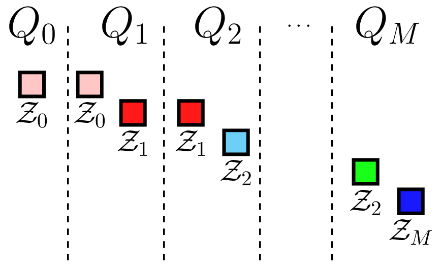
MLMC sampling strategy

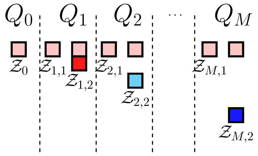
ACV IS sampling strategy

The matrix \(F\) corresponding to this sample scheme is

\[\begin{split}F_{ij}=\begin{cases}\frac{r_i-1}{r_i}\frac{r_j-1}{r_j} & i\neq j\\ \frac{r_i-1}{r_i} & i=j \end{cases}\end{split}\]

Lets apply ACV to the tunable model ensemble

import numpy as np
import matplotlib.pyplot as plt
from functools import partial

from pyapprox.benchmarks import setup_benchmark
from pyapprox import interface
from pyapprox import multifidelity

np.random.seed(2)
shifts = [.1, .2]
benchmark = setup_benchmark(
    "tunable_model_ensemble", theta1=np.pi/2*.95, shifts=shifts)
model = benchmark.fun
model_costs = 10.**(-np.arange(3))
cov = model.get_covariance_matrix()

First let us just use 2 models

print('Two models')
model_ensemble = interface.ModelEnsemble(model.models[:2])
nhf_samples = 10
ntrials = 1000
nsample_ratios = np.array([10])
nsamples_per_model = np.hstack((1, nsample_ratios))*nhf_samples
target_cost = np.dot(model_costs[:2], nsamples_per_model)
est = multifidelity.get_estimator(
    "acvis", benchmark.model_covariance[:2, :2], model_costs[:2],
    benchmark.variable)
means, numerical_var, true_var = \
    multifidelity.estimate_variance(
        model_ensemble, est, target_cost, ntrials, nsample_ratios)

print("Theoretical ACV variance", true_var)
print("Achieved ACV variance", numerical_var)

Two models
Theoretical ACV variance 0.014971109874541333
Achieved ACV variance 0.01617124648499629

Now let us use 3 models

model_ensemble = interface.ModelEnsemble(model.models[:3])
nhf_samples = 10
ntrials = 1000
nsample_ratios = np.array([10, 10])
nsamples_per_model = np.hstack((1, nsample_ratios))*nhf_samples
target_cost = np.dot(model_costs[:3], nsamples_per_model)
est = multifidelity.get_estimator(
    "acvis", benchmark.model_covariance[:3, :3], model_costs[:3],
    benchmark.variable)
means, numerical_var, true_var = \
    multifidelity.estimate_variance(
        model_ensemble, est, target_cost, ntrials, nsample_ratios)

print('Three models')
print("Theoretical ACV variance reduction", true_var)
print("Achieved ACV variance reduction", numerical_var)

Three models
Theoretical ACV variance reduction 0.01475028073510588
Achieved ACV variance reduction 0.014882794078588198

The benefit of using three models over two models depends on the correlation between each low fidelity model and the high-fidelity model. The benefit on using more models also depends on the relative cost of evaluating each model, however here we will just investigate the effect of changing correlation. The following code shows the variance reduction (relative to standard Monte Carlo) obtained using CVMC (not approximate CVMC) using 2 (OCV1) and three models (OCV2). Unlike MLMC and MFMC, ACV-IS will achieve these variance reductions in the limit as the number of samples of the low fidelity models goes to infinity.

from pyapprox.multifidelity.control_variate_monte_carlo import (
    get_control_variate_rsquared
)
theta1 = np.linspace(model.theta2*1.05, model.theta0*0.95, 5)
covs = []
var_reds = []
for th1 in theta1:
    model.theta1 = th1
    covs.append(model.get_covariance_matrix())
    OCV2_var_red = 1-get_control_variate_rsquared(covs[-1])
    # use model with largest covariance with high fidelity model
    idx = [0, np.argmax(covs[-1][0, 1:])+1]
    assert idx == [0, 1] #it will always be the first model
    OCV1_var_red = get_control_variate_rsquared(covs[-1][np.ix_(idx, idx)])
    var_reds.append([OCV2_var_red, OCV1_var_red])
covs = np.array(covs)
var_reds = np.array(var_reds)

fig, axs = plt.subplots(1, 2, figsize=(2*8, 6))
for ii, jj in [[0, 1], [0, 2], [1, 2]]:
    axs[0].plot(theta1, covs[:, ii, jj], 'o-',
                label=r'$\rho_{%d%d}$' % (ii, jj))
axs[1].plot(theta1, var_reds[:, 0], 'o-', label=r'$\mathrm{OCV2}$')
axs[1].plot(theta1, var_reds[:, 1], 'o-', label=r'$\mathrm{OCV1}$')
axs[1].plot(theta1, var_reds[:, 0]/var_reds[:, 1], 'o-',
            label=r'$\mathrm{OCV2/OCV1}$')
axs[0].set_xlabel(r'$\theta_1$')
axs[0].set_ylabel(r'$\mathrm{Correlation}$')
axs[1].set_xlabel(r'$\theta_1$')
axs[1].set_ylabel(r'$\mathrm{Variance\;reduction\;ratio} \; \gamma$')
axs[0].legend()
_ = axs[1].legend()

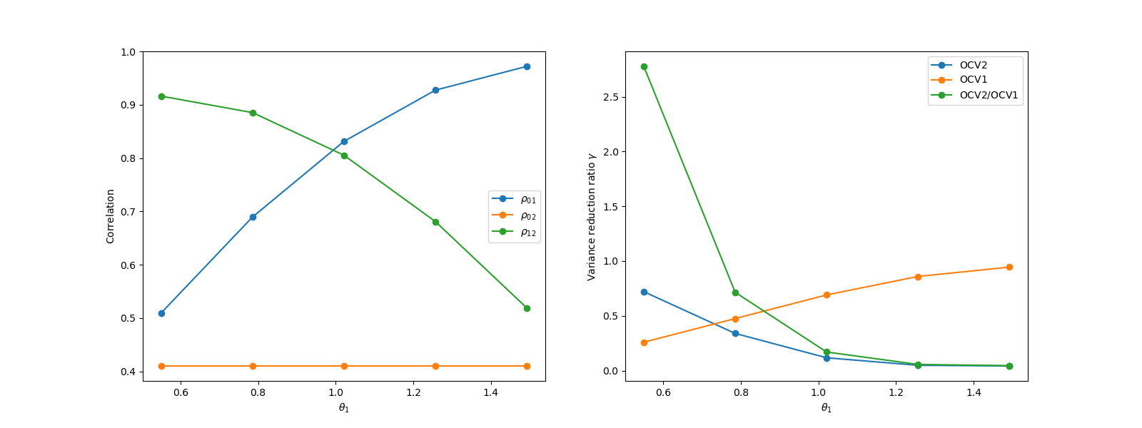
The variance reduction clearly depends on the correlation between all the models.

Let us now compare the variance reduction obtained by MLMC, MFMC and ACV with the MF sampling scheme as we increase the number of samples assigned to the low-fidelity models, while keeping the number of high-fidelity samples fixed. Here we will use the model ensemble

\[f_\alpha(\rv)=\rv^{5-\alpha}, \quad \alpha=0,\ldots,4\]

where each model is the function of a single uniform random variable defined on the unit interval \([0,1]\).

from pyapprox.util.configure_plots import mathrm_labels, mathrm_label
plt.figure()
benchmark = setup_benchmark("polynomial_ensemble")
poly_model = benchmark.fun
cov = poly_model.get_covariance_matrix()
model_costs = np.asarray([10**-ii for ii in range(cov.shape[0])])
nhf_samples = 10
nsample_ratios_base = np.array([2, 4, 8, 16])
cv_labels = mathrm_labels(["OCV-1", "OCV-2", "OCV-4"])
cv_rsquared_funcs = [
    lambda cov: get_control_variate_rsquared(cov[:2, :2]),
    lambda cov: get_control_variate_rsquared(cov[:3, :3]),
    lambda cov: get_control_variate_rsquared(cov)]
cv_gammas = [1-f(cov) for f in cv_rsquared_funcs]
for ii in range(len(cv_gammas)):
    plt.axhline(y=cv_gammas[ii], linestyle='--', c='k')
    xloc = -.35
    plt.text(xloc, cv_gammas[ii]*1.1, cv_labels[ii], fontsize=16)
plt.axhline(y=1, linestyle='--', c='k')
plt.text(xloc, 1, r'$\mathrm{MC}$', fontsize=16)

est_labels = mathrm_labels(["MLMC", "MFMC", "ACVMF"])
estimators = [
    multifidelity.get_estimator("mlmc", cov, model_costs, poly_model.variable),
    multifidelity.get_estimator("mfmc", cov, model_costs, poly_model.variable),
    multifidelity.get_estimator("acvmf", cov, model_costs, poly_model.variable)
]
acv_rsquared_funcs = [est._get_rsquared for est in estimators]

nplot_points = 20
acv_gammas = np.empty((nplot_points, len(acv_rsquared_funcs)))
for ii in range(nplot_points):
    nsample_ratios = np.array([r*(2**ii) for r in nsample_ratios_base])
    acv_gammas[ii, :] = [1-f(cov, nsample_ratios) for f in acv_rsquared_funcs]
for ii in range(len(est_labels)):
    plt.semilogy(np.arange(nplot_points), acv_gammas[:, ii],
                 label=est_labels[ii])
plt.legend()
plt.xlabel(r'$\log_2(r_i)-i$')
_ = plt.ylabel(mathrm_label("Variance reduction ratio ")+r"$\gamma$")

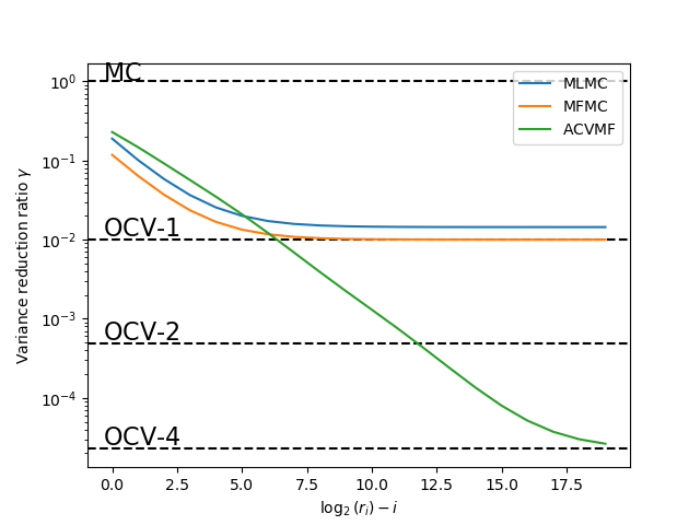
As the theory suggests MLMC and MFMC use multiple models to increase the speed to which we converge to the optimal 2 model CV estimator OCV-2. These two approaches reduce the variance of the estimator more quickly than the ACV estimator, but cannot obtain the optimal variance reduction.

Accelerated Approximate Control Variate Monte Carlo

The recursive estimators work well when the number of low-fidelity samples are smal but ACV can achieve a greater variance reduction for a fixed number of high-fidelity samples. In this section we present an approach called ACV-GMFB that combines the strengths of these methods [BLWLJCP2022].

This estimator differs from the previous recursive estimators because it uses some models as control variates and other models to estimate the mean of these control variates recursively. This estimator optimizes over the best use of models and returns the best model configuration.

Let us add the ACV-GMFB estimator to the previous plot

plt.figure()
cv_labels = mathrm_labels(["OCV-1", "OCV-2", "OCV-4"])
cv_rsquared_funcs = [
    lambda cov: get_control_variate_rsquared(cov[:2, :2]),
    lambda cov: get_control_variate_rsquared(cov[:3, :3]),
    lambda cov: get_control_variate_rsquared(cov)]
cv_gammas = [1-f(cov) for f in cv_rsquared_funcs]
xloc = -.35
for ii in range(len(cv_gammas)):
    plt.axhline(y=cv_gammas[ii], linestyle='--', c='k')
    plt.text(xloc, cv_gammas[ii]*1.1, cv_labels[ii], fontsize=16)
plt.axhline(y=1, linestyle='--', c='k')
plt.text(xloc, 1, mathrm_label("MC"), fontsize=16)

from pyapprox.multifidelity.monte_carlo_estimators import (
    get_acv_recursion_indices
)
est_labels = mathrm_labels(["MLMC", "MFMC", "ACVMF", "ACVGMFB"])
estimator_types = ["mlmc", "mfmc", "acvmf", "acvgmfb"]
estimators = [
    multifidelity.get_estimator(t, cov, model_costs, poly_model.variable)
    for t in estimator_types]
# acvgmfb requires nhf_samples so create wrappers of that does not
estimators[-1]._get_rsquared = partial(
    estimators[-1]._get_rsquared_from_nhf_samples, nhf_samples)
nplot_points = 20
acv_gammas = np.empty((nplot_points, len(estimators)))
for ii in range(nplot_points):
    nsample_ratios = np.array([r*(2**ii) for r in nsample_ratios_base])
    acv_gammas[ii, :] = [1-est._get_rsquared(cov, nsample_ratios)
                         for est in estimators]
for ii in range(len(est_labels)):
    plt.semilogy(np.arange(nplot_points), acv_gammas[:, ii],
                 label=est_labels[ii])
plt.legend()
plt.xlabel(r'$\log_2(r_i)-i$')
_ = plt.ylabel(mathrm_label('Variance reduction ratio ')+ r'$\gamma$')

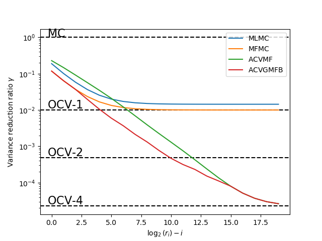
The variance of the best ACV-GMFB still converges to the lowest possible variance. But its variance at small sample sizes is better than ACV-MF and comparable to MLMC.

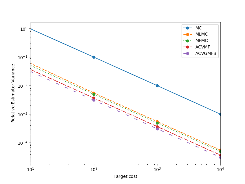
Optimal Sample Allocation

The previous results compared MLMC with MFMC and ACV-MF when the number of high-fidelity samples were fixed. In the following we compare these methods when the number of samples are optimized to minimize the variance of each estimator. We will only use the first 4 models

from pyapprox.util.configure_plots import mathrm_labels, mathrm_label
estimator_types = ["mc", "mlmc", "mfmc", "acvmf", "acvgmfb"]
estimators = [
    multifidelity.get_estimator(t, cov[:4, :4], model_costs[:4], poly_model.variable)
    for t in estimator_types]
est_labels = mathrm_labels(["MC", "MLMC", "MFMC", "ACVMF", "ACVGMFB"])
target_costs = np.array([1e1, 1e2, 1e3, 1e4], dtype=int)
optimized_estimators = multifidelity.compare_estimator_variances(
    target_costs, estimators)

fig, ax = plt.subplots(1, 1, figsize=(8, 6))
multifidelity.plot_estimator_variances(
    optimized_estimators, est_labels, ax,
    ylabel=mathrm_label("Relative Estimator Variance"))
_ = ax.set_xlim(target_costs.min(), target_costs.max())

#fig # necessary for jupyter notebook to reshow plot in new cell

[9.708000e+00 9.930500e+01 9.994940e+02 9.999058e+03] 1

In this example ACVGMFB is the most efficient estimator, i.e. it has a smaller variance for a fixed cost. However this improvement is problem dependent. For other model ensembles another estimator may be more efficient. Modify the above example to use another model to explore this more. The left plot shows the relative costs of evaluating each model using the ACVMF sampling strategy. Compare this to the MLMC sample allocation. Also edit above code to plot the MFMC sample allocation.

Before this tutorial ends it is worth noting that a section of the MLMC literature explores adaptive methods which do not assume there is a fixed high-fidelity model but rather attempt to balance the estimator variance with the deterministic bias. These methods add a higher-fidelity model, e.g. a finer finite element mesh, when the variance is made smaller than the bias. We will not explore this here, but an example of this is shown in the tutorial on multi-index collocation.

References

[GGEJJCP2020] (1,2)

A generalized approximate control variate framework for multifidelity uncertainty quantification, Journal of Computational Physics, 408:109257, 2020.

[BLWLJCP2022]

On the optimization of approximate control variates with parametrically defined estimators, Journal of Computational Physics,451:110882, 2022