Approximate Control Variate Monte Carlo

This tutorial builds upon Control Variate Monte Carlo and describes how to implement and deploy approximate control variate Monte Carlo (ACVMC) sampling to compute expectations of model output from multiple low-fidelity models with unknown means.

CVMC is often not useful for practical analysis of numerical models because typically the mean of the lower fidelity model, i.e. ${\mu }_{\mathit{\kappa }}$, is unknown and the cost of the lower fidelity model is non trivial. These two issues can be overcome by using approximate control variate Monte Carlo.

Let the cost of the high fidelity model per sample be $C_{\alpha }$ and let the cost of the low fidelity model be $C_{\kappa }$. Now lets use $N$ samples to estimate $Q_{\mathit{\alpha },N}$ and $Q_{\mathit{\kappa },N}$ and these $N$ samples plus another $(r-1)N$ samples to estimate ${\mu }_{\mathit{\kappa }}$ so that

$$Q_{\mathit{\alpha },N,r}^{\text{ACV}}=Q_{\mathit{\alpha },N}+\eta (Q_{\mathit{\kappa },N}-{\mu }_{\mathit{\kappa },N,r})$$

and

$${\mu }_{\mathit{\kappa },N,r}=\frac{1}{rN}\sum _{i=1}^{rN}{Q}_{\mathit{\kappa }}$$

With this sampling scheme we have

$$\begin{array}{rl}{Q}_{\mathit{\kappa },N}-{\mu }_{\mathit{\kappa },N,r}& =\frac{1}{N}\sum _{i=1}^N{f}_{\mathit{\kappa }}^{(i)}-\frac{1}{rN}\sum _{i=1}^{rN}{f}_{\mathit{\kappa }}^{(i)}\\ & =\frac{1}{N}\sum _{i=1}^N{f}_{\mathit{\kappa }}^{(i)}-\frac{1}{rN}\sum _{i=1}^N{f}_{\mathit{\kappa }}^{(i)}-\frac{1}{rN}\sum _{i=N}^{rN}{f}_{\mathit{\kappa }}^{(i)}\\ & =\frac{r-1}{rN}\sum _{i=1}^N{f}_{\mathit{\kappa }}^{(i)}-\frac{1}{rN}\sum _{i=N}^{rN}{f}_{\mathit{\kappa }}^{(i)}\end{array}$$

where for ease of notation we write $r_{\mathit{\kappa }}N$ and $\lfloor r_{\mathit{\kappa }}N\rfloor$ interchangibly. Using the above expression yields

$$\begin{array}{rl}\mathbb{V}\left[(Q_{\mathit{\kappa },N}-{\mu }_{\mathit{\kappa },N,r})\right]& =\mathbb{E}\left[{(\frac{r-1}{rN}\sum _{i=1}^N{f}_{\mathit{\kappa }}^{(i)}-\frac{1}{rN}\sum _{i=N}^{rN}{f}_{\mathit{\kappa }}^{(i)})}^2\right]\\ & =\frac{(r-1{)}^2}{r^2{N}^2}\sum _{i=1}^N\mathbb{V}\left[f_{\mathit{\kappa }}^{(i)}\right]+\frac{1}{r^2{N}^2}\sum _{i=N}^{rN}\mathbb{V}\left[f_{\mathit{\kappa }}^{(i)}\right]\\ & =\frac{(r-1{)}^2}{r^2{N}^2}N\mathbb{V}\left[f_{\mathit{\kappa }}\right]+\frac{1}{r^2{N}^2}(r-1)N\mathbb{V}\left[f_{\mathit{\kappa }}\right]\\ & =\frac{r-1}{r}\frac{\mathbb{V}\left[f_{\mathit{\kappa }}\right]}{N}\end{array}$$

where we have used the fact that since the samples used in the first and second term on the first line are not shared, the covariance between these terms is zero. Also we have

$$\mathbb{C}\text{ov}[Q_{\mathit{\alpha },N},(Q_{\mathit{\kappa },N}-{\mu }_{\mathit{\kappa },N,r})]=\mathbb{C}\text{ov}[\frac{1}{N}\sum _{i=1}^N{f}_{\mathit{\alpha }}^{(i)},\frac{r-1}{rN}\sum _{i=1}^N{f}_{\mathit{\kappa }}^{(i)}-\frac{1}{rN}\sum _{i=N}^{rN}{f}_{\mathit{\kappa }}^{(i)}]$$

The correlation between the estimators $\frac{1}{N}\sum _{i=1}^N{Q}_{\mathit{\alpha }}$ and $\frac{1}{rN}\sum _{i=N}^{rN}{Q}_{\mathit{\kappa }}$ is zero because the samples used in these estimators are different for each model. Thus

$$\begin{array}{rl}\mathbb{C}\text{ov}[Q_{\mathit{\alpha },N},(Q_{\mathit{\kappa },N}-{\mu }_{\mathit{\kappa },N,r})]& =\mathbb{C}\text{ov}[\frac{1}{N}\sum _{i=1}^N{f}_{\mathit{\alpha }}^{(i)},\frac{r-1}{rN}\sum _{i=1}^N{f}_{\mathit{\kappa }}^{(i)}]\\ & =\frac{r-1}{r}\frac{\mathbb{C}\text{ov}[f_{\mathit{\alpha }},f_{\mathit{\kappa }}]}{N}\end{array}$$

Recalling the variance reduction of the CV estimator using the optimal $\eta$ is

$$\begin{array}{rl}\gamma & =1-\frac{\mathbb{C}\text{ov}{[Q_{\mathit{\alpha },N},(Q_{\mathit{\kappa },N}-{\mu }_{\mathit{\kappa },N,r})]}^2}{\mathbb{V}\left[(Q_{\mathit{\kappa },N}-{\mu }_{\mathit{\kappa },N,r})\right]\mathbb{V}\left[Q_{\mathit{\alpha },N}\right]}\\ & =1-\frac{N^{-2}\frac{(r-1{)}^2}{r^2}\mathbb{C}\text{ov}[f_{\mathit{\alpha }},f_{\mathit{\kappa }}]}{N^{-1}\frac{r-1}{r}\mathbb{V}\left[f_{\mathit{\kappa }}\right]N^{-1}\mathbb{V}\left[f_{\mathit{\alpha }}\right]}\\ & =1-\frac{r-1}{r}\mathbb{C}\text{or}{[f_{\mathit{\alpha }},f_{\mathit{\kappa }}]}^2\end{array}$$

which is found when

$$\begin{array}{rl}\eta & =-\frac{\mathbb{C}\text{ov}[Q_{\mathit{\alpha },N},(Q_{\mathit{\kappa },N}-{\mu }_{\mathit{\kappa },N,r})]}{\mathbb{V}\left[(Q_{\mathit{\kappa },N}-{\mu }_{\mathit{\kappa },N,r})\right]}\\ & =-\frac{N^{-1}\frac{r-1}{r}\mathbb{C}\text{ov}[f_{\mathit{\alpha }},f_{\mathit{\kappa }}]}{N^{-1}\frac{r-1}{r}\mathbb{V}\left[f_{\mathit{\kappa }}\right]}\\ & =-\frac{\mathbb{C}\text{ov}[f_{\mathit{\alpha }},f_{\mathit{\kappa }}]}{\mathbb{V}\left[f_{\mathit{\kappa }}\right]}\end{array}$$

Lets setup the problem and compute an ACV estimate of $\mathbb{E}\left[f_0\right]$

import numpy as np
import matplotlib.pyplot as plt

from pyapprox.benchmarks import setup_benchmark

np.random.seed(1)
shifts = [.1, .2]
benchmark = setup_benchmark(
    "tunable_model_ensemble", theta1=np.pi/2*.95, shifts=shifts)
model = benchmark.fun
exact_integral_f0 = benchmark.means[0]

Before proceeding to estimate the mean using ACVMV we must first define how to generate samples to estimate $Q_{\mathit{\alpha },N}$ and ${\mu }_{\mathit{\kappa },N,r}$. To do so clearly we must first introduce some additional notation. Let ${\mathcal{Z}}_0$ be the set of samples used to evaluate the high-fidelity model and let ${\mathcal{Z}}_{\alpha }={\mathcal{Z}}_{\alpha ,1}\cup {\mathcal{Z}}_{\alpha ,2}$ be the samples used to evaluate the low fidelity model. Using this notation we can rewrite the ACV estimator as

$$Q_{\mathit{\alpha },\mathcal{Z}}^{\text{ACV}}=Q_{\mathit{\alpha },{\mathcal{Z}}_0}+\eta (Q_{\mathit{\kappa },{\mathcal{Z}}_{\alpha ,1}}-{\mu }_{\mathit{\kappa },{\mathcal{Z}}_{\alpha ,2}})$$

where $\mathcal{Z}=\bigcup _{\alpha =0}^M{Z}_{\alpha }$. The nature of these samples can be changed to produce different ACV estimators. Here we choose ${\mathcal{Z}}_{\alpha ,1}\cap {\mathcal{Z}}_{\alpha ,2}=\mathrm{\varnothing }$ and ${\mathcal{Z}}_{\alpha ,1}={\mathcal{Z}}_{\mathcal{0}}$. That is we use the set a common set of samples to compute the covariance between all the models and a second independent set to estimate the lower fidelity mean. The sample partitioning for $M$ models is shown in the following Figure. We call this scheme the ACV IS sampling strategy where IS indicates that the second sample set ${\mathcal{Z}}_{\alpha ,2}$ assigned to each model are not shared.

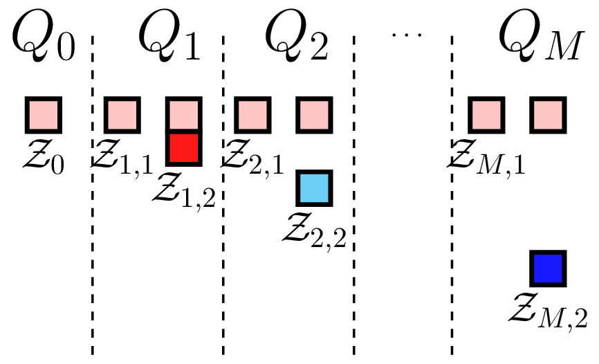
ACV IS sampling strategy

The following code generates samples according to this strategy

from pyapprox import multifidelity
model_costs = 10.**(-np.arange(3))
est = multifidelity.get_estimator(
    "acvis", benchmark.model_covariance[:2, :2], model_costs[:2],
    benchmark.variable)
est.nsamples_per_model = np.array([10, 100])
samples_per_model, partition_indices_per_model = \
    est.generate_sample_allocations()

print(partition_indices_per_model)
samples_shared = samples_per_model[0]
samples_lf_only = samples_per_model[1][:, partition_indices_per_model[1] == 1]

[array([0., 0., 0., 0., 0., 0., 0., 0., 0., 0.]), array([0., 0., 0., 0., 0., 0., 0., 0., 0., 0., 1., 1., 1., 1., 1., 1., 1.,
       1., 1., 1., 1., 1., 1., 1., 1., 1., 1., 1., 1., 1., 1., 1., 1., 1.,
       1., 1., 1., 1., 1., 1., 1., 1., 1., 1., 1., 1., 1., 1., 1., 1., 1.,
       1., 1., 1., 1., 1., 1., 1., 1., 1., 1., 1., 1., 1., 1., 1., 1., 1.,
       1., 1., 1., 1., 1., 1., 1., 1., 1., 1., 1., 1., 1., 1., 1., 1., 1.,
       1., 1., 1., 1., 1., 1., 1., 1., 1., 1., 1., 1., 1., 1., 1.])]

Now lets plot the samples assigned to each model.

fig, ax = plt.subplots()
ax.plot(samples_shared[0, :], samples_shared[1, :], 'ro', ms=12,
        label=r'$\mathrm{Low\ and\  high\  fidelity\  models}$')
ax.plot(samples_lf_only[0, :], samples_lf_only[1, :], 'ks',
        label=r'$\mathrm{Low\  fidelity\  model\ only}$')
ax.set_xlabel(r'$z_1$')
ax.set_ylabel(r'$z_2$', rotation=0)
_ = ax.legend(loc='upper left')

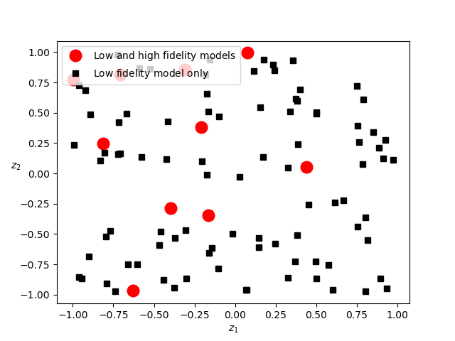
The high-fidelity model is only evaluated on the red dots. Now lets use these samples to estimate the mean of $f_0$.

values_per_model = []
for ii in range(len(samples_per_model)):
    values_per_model.append(model.models[ii](samples_per_model[ii]))

acv_mean = est.estimate_from_values_per_model(
    values_per_model, partition_indices_per_model)

print('MC difference squared =', (
    values_per_model[0].mean()-exact_integral_f0)**2)
print('ACVMC difference squared =', (acv_mean-exact_integral_f0)**2)

MC difference squared = 0.1663308327274871
ACVMC difference squared = 0.010697826122695035

Note here we have arbitrarily set the number of high fidelity samples $N$ and the ratio $r$. In practice one should choose these in one of two ways: (i) for a fixed budget choose the free parameters to minimize the variance of the estimator; or (ii) choose the free parameters to achieve a desired MSE (variance) with the smallest computational cost. Note the cost of computing the two model ACV estimator is

$$C_{\mathrm{cv}}=N{C}_{\alpha }+r_{\mathit{\kappa }}N{C}_{\kappa }$$

Now lets compute the variance reduction for different sample sizes

from pyapprox import interface
model_ensemble = interface.ModelEnsemble(model.models[:2])
nhf_samples = 10
ntrials = 1000
nsample_ratios = np.array([10])
nsamples_per_model = np.hstack((1, nsample_ratios))*nhf_samples
target_cost = np.dot(model_costs[:2], nsamples_per_model)
means, numerical_var, true_var = \
    multifidelity.estimate_variance(
        model_ensemble, est, target_cost, ntrials, nsample_ratios)

print("Theoretical ACV variance", true_var)
print("Achieved ACV variance", numerical_var)

Theoretical ACV variance 0.014971109874541333
Achieved ACV variance 0.01617124648499629

Let us also plot the distribution of these estimators

fig, ax = plt.subplots()
ax.hist(means[:, 0], bins=ntrials//100, density=True, alpha=0.5,
        label=r'$Q_{0, N}$')
ax.hist(means[:, 1], bins=ntrials//100, density=True, alpha=0.5,
        label=r'$Q_{0, N, %d}^\mathrm{CV}$' % nsample_ratios[0])

nsample_ratios = np.array([100])
nsamples_per_model = np.hstack((1, nsample_ratios))*nhf_samples
target_cost = np.dot(model_costs[:2], nsamples_per_model)
means, numerical_var, true_var = \
    multifidelity.estimate_variance(
        model_ensemble, est, target_cost, ntrials, nsample_ratios)
ax.hist(means[:, 1], bins=ntrials//100, density=True, alpha=0.5,
        label=r'$Q_{0, N, %d}^\mathrm{CV}$' % nsample_ratios[0])
ax.axvline(x=0, c='k', label=r'$E[Q_0]$')
_ = ax.legend(loc='upper left')

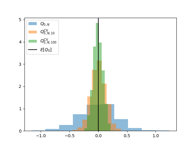
For a fixed number of high-fidelity evaluations $N$ the ACVMC variance reduction will converge to the CVMC variance reduction. Try changing $N$.

References

[GGEJJCP2020]

A generalized approximate control variate framework for multifidelity uncertainty quantification, Journal of Computational Physics, 408:109257, 2020.