Multi-index Stochastic Collocation

This tutorial describes how to implement and deploy multi-index collocation to construct a surrogate of the output of a high-fidelity model using a set of lower-fidelity models of lower accuracy and cost.

Despite the improved efficiency of surrogate methods relative to MC sampling, building a surrogate can still be prohibitively expensive for high-fidelity simulation models. Fortunately, a selection of models of varying fidelity and computational cost are typically available for many applications. For example, aerospace models span fluid dynamics, structural and thermal response, control systems, etc.

Leveraging an ensemble of models can facilitate significant reductions in the overall computational cost of UQ, by integrating the predictions of quantities of interest (QoI) from multiple sources.

\[\begin{split}\frac{\partial u}{\partial t}(x,t,\rv) + \nabla u(x,t,\rv)-\nabla\cdot\left[k(x,\rv) \nabla u(x,t,\rv)\right] &= g(x,t) \qquad\qquad (x,t,\rv)\in D\times [0,1]\times\rvdom\\ u(x,t,\rv)&=0 \qquad\qquad\qquad (x,t,\rv)\in \partial D\times[0,1]\times\rvdom\end{split}\]

with forcing \(g(x,t)=(1.5+\cos(2\pi t))\cos(x_1)\), and subject to the initial condition \(u(x,0,\rv)=0\). Following [NTWSIAMNA2008], we model the diffusivity \(k\) as a random field represented by the Karhunen-Loeve (like) expansion (KLE)

\[\log(k(x,\rv)-0.5)=1+\rv_1\left(\frac{\sqrt{\pi L}}{2}\right)^{1/2}+\sum_{k=2}^d \lambda_k\phi(x)\rv_k,\]

with

\[\begin{split}\lambda_k=\left(\sqrt{\pi L}\right)^{1/2}\exp\left(-\frac{(\lfloor\frac{k}{2}\rfloor\pi L)^2}{4}\right) k>1, \qquad\qquad \phi(x)= \begin{cases} \sin\left(\frac{(\lfloor\frac{k}{2}\rfloor\pi x_1)}{L_p}\right) & k \text{ even}\,,\\ \cos\left(\frac{(\lfloor\frac{k}{2}\rfloor\pi x_1)}{L_p}\right) & k \text{ odd}\,. \end{cases}\end{split}\]

where \(L_p=\max(1,2L_c)\), \(L=\frac{L_c}{L_p}\) and \(L_c=0.5\).

We choose a random field which is effectively one-dimensional so that the error in the finite element solution is more sensitive to refinement of the mesh in the \(x_1\)-direction than to refinement in the \(x_2\)-direction.

The advection diffusion equation is solved using linear finite elements and implicit backward-Euler timestepping implemented using Fenics. In the following we will show how solving the PDE with varying numbers of finite elements and timesteps can reduce the cost of approximating the quantity of interest

\[f(\rv)=\int_D u(\rv)\frac{1}{2\pi\sigma^2}\exp\left(-\frac{\lVert x-x^\star \rVert_2^2}{\sigma^2}\right)\,dx,\]

where \(x^\star=(0.3,0.5)\) and \(\sigma=0.16\).

Lets first consider a simple example with one unknown parameter. The following sets up the problem

import numpy as np
import pyapprox as pya
from scipy.stats import uniform
from pyapprox.models.wrappers import MultiLevelWrapper
import matplotlib.pyplot as plt

nmodels  = 3
nrandom_vars, corr_len = 1, 1/2
max_eval_concurrency = 1
from pyapprox.benchmarks.benchmarks import setup_benchmark
benchmark = setup_benchmark(
    'multi_level_advection_diffusion',nvars=nrandom_vars,corr_len=corr_len,
    max_eval_concurrency=max_eval_concurrency)
model = benchmark.fun
variable = benchmark.variable

Now lets us plot each model as a function of the random variable

lb,ub = variable.get_statistics('interval',alpha=1)[0]
nsamples = 10
random_samples = np.linspace(lb,ub,nsamples)[np.newaxis,:]
config_vars = np.arange(nmodels)[np.newaxis,:]
samples = pya.get_all_sample_combinations(random_samples,config_vars)
values = model(samples)
values = np.reshape(values,(nsamples,nmodels))

import dolfin as dl
plt.figure(figsize=(nmodels*8,2*6))
config_samples = benchmark['multi_level_model'].map_to_multidimensional_index(config_vars)
for ii in range(nmodels):
    nx,ny = model.base_model.get_mesh_resolution(config_samples[:2,ii])
    dt = model.base_model.get_timestep(config_samples[2,ii])
    mesh = dl.RectangleMesh(dl.Point(0, 0),dl.Point(1, 1), nx, ny)
    plt.subplot(2,nmodels,ii+1)
    dl.plot(mesh)
    label=r'$f_%d$'%ii
    if ii==0:
        ax = plt.subplot(2,nmodels,nmodels+ii+1)
    else:
        plt.subplot(2,nmodels,nmodels+ii+1,sharey=ax)
    plt.plot(random_samples[0,:],values[:,ii],label=label)
    if ii>0:
        label=r'$f_%d-f_%d$'%(ii,ii-1)
        plt.plot(random_samples[0,:],values[:,ii]-values[:,ii-1],label=label)
    plt.legend()
#plt.show()

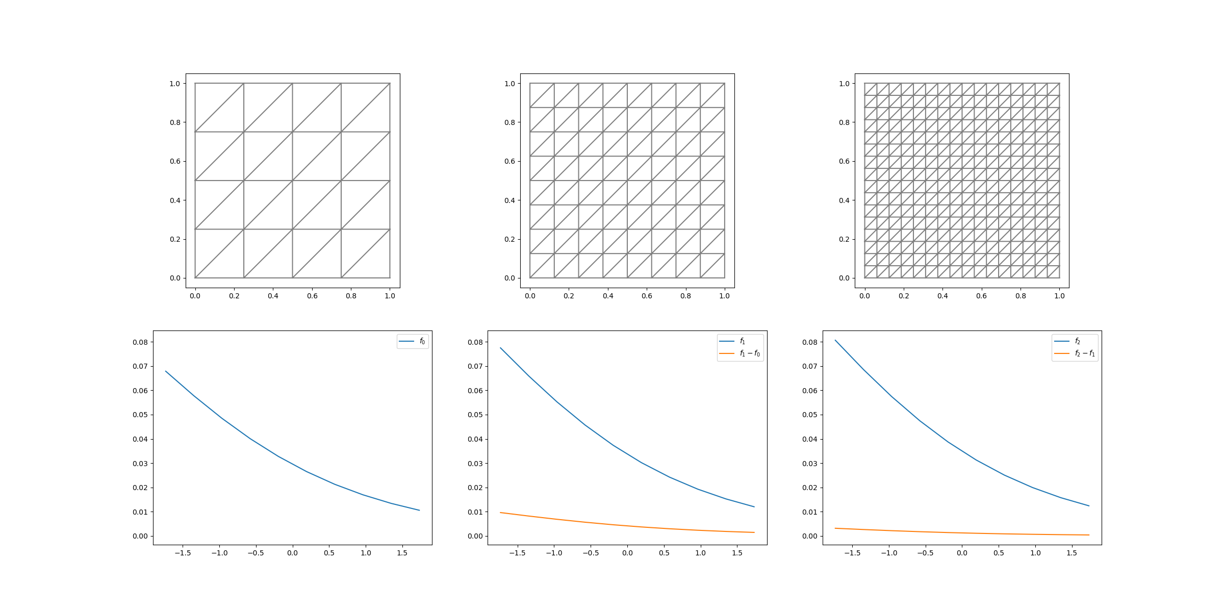
The first row shows the spatial mesh of each model and the second row depicts the model response and the discrepancy between two consecutive models. The difference between the model output decreases as the resolution of the mesh is increased. Thus as the cost of the model increases (with increasing resolution) we need less samples to resolve

Lets now construct a multi-level approximation with the same model but more random variables. We will need a model that takes in only 1 configuration variable. We can do this with the MultiLevelWrapper. Here we will call another benchmark which is the same advection diffusion problem but with the multi-level wrapper already in place. Here the levels have the one-to-one mapping [0,1,2,…]->[[0,0,0],[1,1,1],[2,2,2],…]

nrandom_vars = 10
benchmark = setup_benchmark(
    'multi_level_advection_diffusion',nvars=nrandom_vars,corr_len=corr_len,
    max_eval_concurrency=max_eval_concurrency)
model = benchmark.fun
variable = benchmark.variable

First define the levels of the multi-level model we will use. Will will skip level 0 and use levels 1,2, and 3. Thus we must define a transformation that converts the sparse grid indices starting at 0 to these levels. We can do this with

from pyapprox.adaptive_sparse_grid import ConfigureVariableTransformation
level_indices = [[1,2,3,4]]
config_var_trans = ConfigureVariableTransformation(level_indices)

Before building the sparse grid approximation let us define a callback to compute the error and total cost at each step of the sparse grid construction. To do this we will precompute some validation data. Specifically we will evaluate the model using a discretization on level higher than the discretization used to construct the sparse grid. We first generate random samples and then append in the configure variable to each of these samples

validation_level = level_indices[0][-1]+1
nvalidation_samples = 20
random_validation_samples = pya.generate_independent_random_samples(variable,nvalidation_samples)
validation_samples = np.vstack([random_validation_samples,validation_level*np.ones((1,nvalidation_samples))])
validation_values = model(validation_samples)

#print(model.work_tracker.costs)

errors,total_cost = [],[]
def callback(approx):
    approx_values=approx.evaluate_using_all_data(
        validation_samples)
    error = np.linalg.norm(
        validation_values-approx_values)/np.sqrt(validation_samples.shape[1])
    errors.append(error)
    total_cost.append(approx.num_equivalent_function_evaluations)

We can add this callback to the sparse grid options. We define max_nsamples to be the total cost used to evaluate all samples in the sparse grid

max_nsamples = 100
from pyapprox.multifidelity import adaptive_approximate_multi_index_sparse_grid
cost_function = model.cost_function
def cost_function(multilevel_config_sample):
    config_sample = benchmark.multi_level_model.map_to_multidimensional_index(
        multilevel_config_sample)
    nx,ny=model.base_model.get_mesh_resolution(config_sample[:2])
    dt = model.base_model.get_timestep(config_sample[2])
    ndofs = nx*ny*model.base_model.final_time/dt
    return ndofs/1e5

options = {'config_var_trans':config_var_trans,'max_nsamples':max_nsamples,
           'config_variables_idx':nrandom_vars,'verbose':0,
           'cost_function':cost_function,
           'max_level_1d':[np.inf]*nrandom_vars+[
               len(level_indices[0])-1]*len(level_indices),
           'callback':callback}

Now lets us build the sparse grid

sparse_grid = adaptive_approximate_multi_index_sparse_grid(
    model,variable.all_variables(),options)

# #%%
# #Lets plot the errors
# fig, ax = plt.subplots(1,1,figsize=(8,6))
# plt.loglog(total_cost,errors)
# plt.show()

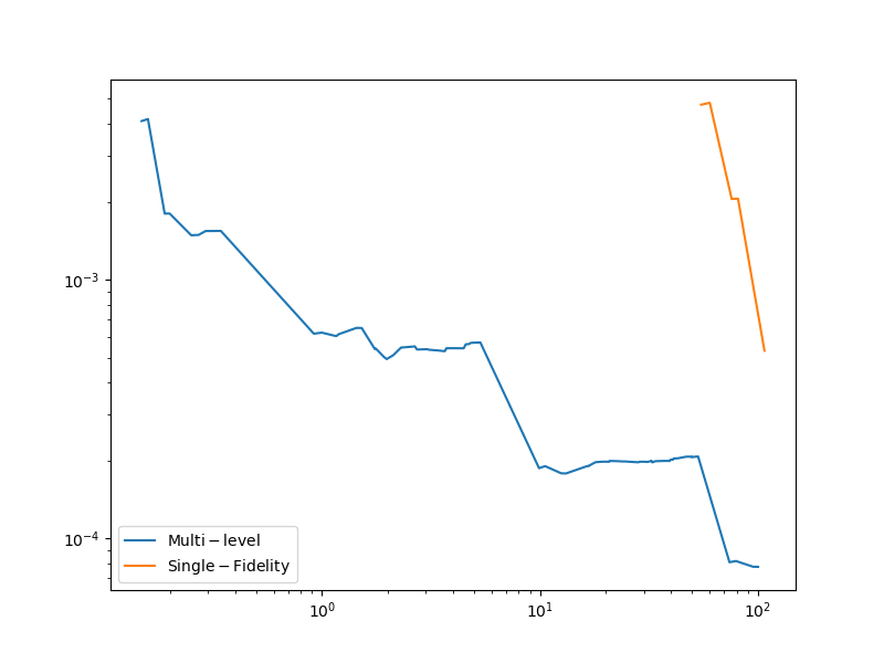
Now lets build a single fidelity approximation

multi_level_indices = level_indices.copy()
level_indices = [[level_indices[0][-1]]]
config_var_trans = ConfigureVariableTransformation(level_indices)
#cost_function = model.cost_function
options = {'config_var_trans':config_var_trans,'max_nsamples':max_nsamples,
           'config_variables_idx':nrandom_vars,'verbose':0,
           'cost_function':cost_function,
           'max_level_1d':[np.inf]*nrandom_vars+[
               len(level_indices[0])-1]*len(level_indices),
           'callback':callback}

Now lets us build the sparse grid. First reset the callback counters and save the previous errors

multi_level_errors,multi_level_total_cost = errors.copy(), total_cost.copy()
errors,total_cost = [],[]
sparse_grid = adaptive_approximate_multi_index_sparse_grid(
    model,variable.all_variables(),options)

Lets plot the errors

fig, ax = plt.subplots(1,1,figsize=(8,6))
plt.loglog(multi_level_total_cost,multi_level_errors,
           label=r'$\mathrm{Multi}-\mathrm{level}$')
plt.loglog(total_cost,errors,
           label=r'$\mathrm{Single}-\mathrm{Fidelity}$')
plt.legend()

Out:

<matplotlib.legend.Legend object at 0x12fb034d0>

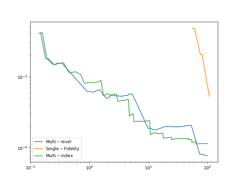
Now lets build a multi-index approximation of the same model but now with more random variables. We again create the same benchmark but this time one that allows us to vary the two spatial mesh resolutions and the timestep independently

benchmark = setup_benchmark(
    'multi_index_advection_diffusion',nvars=nrandom_vars,corr_len=corr_len,
    max_eval_concurrency=max_eval_concurrency)
model = benchmark.fun
variable = benchmark.variable

Again we define the ConfigureVariableTransformation and define the appropriate options. Notice the different in max_level_1d. (print it; it should be longer than the single fidelity and multi-level versions)

from pyapprox.adaptive_sparse_grid import ConfigureVariableTransformation
level_indices = multi_level_indices*3
config_var_trans = ConfigureVariableTransformation(level_indices)

from pyapprox.multifidelity import adaptive_approximate_multi_index_sparse_grid
#cost_function = model.cost_function
def cost_function(config_sample):
    nx,ny=model.base_model.get_mesh_resolution(config_sample[:2])
    dt = model.base_model.get_timestep(config_sample[2])
    ndofs = nx*ny*model.base_model.final_time/dt
    return ndofs/1e5
options = {'config_var_trans':config_var_trans,'max_nsamples':max_nsamples,
           'config_variables_idx':nrandom_vars,'verbose':0,
           'cost_function':cost_function,
           'max_level_1d':[np.inf]*nrandom_vars+[
               len(level_indices[0])-1]*len(level_indices),
           'callback':callback}

single_fidelity_errors,single_fidelity_total_cost = errors.copy(), total_cost.copy()
errors,total_cost = [],[]
sparse_grid = adaptive_approximate_multi_index_sparse_grid(
    model,variable.all_variables(),options)

Lets plot the errors

fig, ax = plt.subplots(1,1,figsize=(8,6))
plt.loglog(multi_level_total_cost,multi_level_errors,
           label=r'$\mathrm{Multi}-\mathrm{level}$')
plt.loglog(single_fidelity_total_cost,single_fidelity_errors,
           label=r'$\mathrm{Single}-\mathrm{Fidelity}$')
plt.loglog(total_cost,errors,label=r'$\mathrm{Multi}-\mathrm{index}$')
plt.legend()
plt.show()

References

TJWGSIAMUQ2015

Teckentrup, A. and Jantsch, P. and Webster, C. and Gunzburger, M. A Multilevel Stochastic Collocation Method for Partial Differential Equations with Random Input Data. SIAM/ASA Journal on Uncertainty Quantification, 3(1), 1046-1074, 2015.

HNTTCMAME2016

Haji-Ali, A. and Nobile, F. and Tamellini, L. and Tempone, R. Multi-Index Stochastic Collocation for random PDEs. Computer Methods in Applied Mechanics and Engineering, 306, 95-122, 2016.

JEGGIJNME2020

Jakeman, J.D., Eldred, M.S., Geraci, G., Gorodetsky, A. Adaptive multi-index collocation for uncertainty quantification and sensitivity analysis. Int J Numer Methods Eng. 2020; 121: 1314– 1343.