Numerical Approximations of Governing Equations

This tutorial discusses the effect of numerically solving governing equations on model uncertainty. The following focuses on models based upon partial differential equations, but the points raised below apply to a much broader class of numerical models.

Partial Differential Equations

We seek to quantify uncertainty in a broad class of stochastic partial differential equations (PDE). Let $D\subset\mathbb{R}^\ell$, for $\ell=1,2,$ or $3$ and $\text{dim}(D)=\ell$, be a physical domain; $T>0$ be a real number; and $\rvdom\subseteq \mathbb{R}^{d}$, for $d\geq 1$ and $\text{dim}(\rvdom)=d$, be the stochastic space. The PDE is defined as

$$\begin{split}\left\{ \begin{array} {ll} u_t(x,t,\rv) = \mathcal{L}(u), &\\ \mathcal{B}(u(x, t, \rv)) = 0, & \\ u(x, 0, \rv) = u_0(x, \rv), & %% D\times\{t=0\}\times \rvdom \end{array} \right.\end{split}$$

where $t$ is the time, $x=(x_1,\dots,x_\ell)$ is the physical coordinate, $\mathcal{L}$ is a (nonlinear) differential operator, $\mathcal{B}$ is the boundary condition operator, $u_0$ is the initial condition, and $\rv=(\rv_1,\dots,\rv_{d})\in \rvdom$ are a set of random variables characterizing the random inputs to the governing equation. The solution $u \in V$ is a vector-valued stochastic quantity

$$u:\bar{D}\times[0,T]\times \rvdom\to\mathbb{R}^{n},$$

for some suitable function space $V$ and where $\bar{D} = D \times \partial D$ is the closure of the interior domain. As an example, $u(x,t, \rv)$ can be a vector of temperatures, pressures, and velocities for a specific location in the domain $x$, specific time $t$, and for a specific realization $\rv$ of the stochastic variable $\rv$.

In this tutorial we will consider the following model of advection-diffusion

$$\begin{split}\frac{\partial u}{\partial t}(x,t,\rv) + \nabla u(x,t,\rv)-\nabla\cdot\left[k(x,\rv) \nabla u(x,t,\rv)\right] &=g(x,t) \qquad\qquad (x,t,\rv)\in D\times [0,1]\times\rvdom\\ u(x,t,\rv)&=0 \qquad\qquad\qquad (x,t,\rv)\in \partial D\times[0,1]\times\rvdom\end{split}$$

with forcing $g(x,t)=(1.5+\cos(2\pi t))\cos(x_1)$, and subject to the initial condition $u(x,0,\rv)=0$. Following [NTWSIAMNA2008], we model the diffusivity $k$ as a random field represented by the Karhunen-Loeve (like) expansion (KLE)

$$\log(k(x,\rv)-0.5)=1+\rv_1\left(\frac{\sqrt{\pi L}}{2}\right)^{1/2}+\sum_{k=2}^d \lambda_k\phi(x)\rv_k,$$

with

$$\begin{split}\lambda_k=\left(\sqrt{\pi L}\right)^{1/2}\exp\left(-\frac{(\lfloor\frac{k}{2}\rfloor\pi L)^2}{4}\right) k>1, \qquad\qquad \phi(x)= \begin{cases} \sin\left(\frac{(\lfloor\frac{k}{2}\rfloor\pi x_1)}{L_p}\right) & k \text{ even}\,,\\ \cos\left(\frac{(\lfloor\frac{k}{2}\rfloor\pi x_1)}{L_p}\right) & k \text{ odd}\,. \end{cases}\end{split}$$

where $L_p=\max(1,2L_c)$, $L=\frac{L_c}{L_p}$ and $L_c=0.5$.

We choose a random field which is effectively one-dimensional so that the error in the finite element solution is more sensitive to refinement of the mesh in the $x_1$-direction than to refinement in the $x_2$-direction.

Quantities of Interest

Often, one is more interested in quantifying uncertainty in a particular functional of the solution, called the quantity of interest (QoI), rather than the full solution. Let

$$F\left[u\right]: V \rightarrow \mathbb{R}^{q}, \qquad q>0$$

be such a function, where $F$ is typically a continuous and bounded functional. Then, we are interested in estimating statistics of the function

$$f(\rv)=F[u(\cdot,\rv)] : \Gamma \to \mathbb{R}^{q}.$$

which assigns the value of the quantity of interest $F[u]$ to each realization of the random variables $\rv$. The above expression allows us to express the QoI as a function of the random variables without needed to explicitly state the dependence of the QoI on the PDE solution.

For the advection-diffusion model we consider the quantity of interest

$$f(\rv)=\int_D u(\rv)\frac{1}{2\pi\sigma^2}\exp\left(-\frac{\lVert x-x^\star \rVert_2^2}{\sigma^2}\right)\,dx,$$

where $x^\star=(0.3,0.5)$ and $\sigma=0.16$.

Numerical Approximations

For most, if not all, practical applications, the solutions of the governing equations and statistics of the resulting QoI cannot be computed analytically and numerical approximations must be employed. In the following we will consider finite element approximations, but other approaches such as finite volume and finite difference can also be used.

Given a set of governing equations, we assume access to a PDE solver that approximates the solution $u$ of these equations for a given fixed $\rv$. We also assume this solver has a set of hyper-parameters — mesh size, time step, maximum number of iterations, convergence tolerance, etc. — which can be used to estimate the QoI $f$ at varying accuracy and cost. Differing settings for these hyper-parameters produces simulations of varying fidelities (resolution). We refer to approaches that leverage only one model or solver setting as single-fidelity methods and approaches that leverage multiple models and settings as multi-fidelity methods.

The accuracy and cost of a model is often determined by a set of solver parameters, such as mesh size, time step, tolerances of numerical solvers. Let ${n_\ai}$ denote the number of such parameters for a given model. Furthermore let $l_{\ai_i} \in \mathbb{N}$ denote the number of values that each solver parameter can assume, such that the multi-index $\ai=(\ai_1,\ldots,\ai_{n_\ai})\in\mathbb{N}^{n_\ai}$, $\ai_i\in \mathcal{M}_{\ai_i}=\{1,\ldots,l_{\ai_i}\}$ can be used to index specific values of the solver parameters. Finally let $f_\ai(\rv)$ to denote a single-fidelity physical approximation of the QoI $f(\rv)$ using the solver parameters indexed by $\ai$.

The advection-diffusion equation is solved with Fenics using the Galerkin finite element method with linear finite elements and the implicit backward-Euler time-stepping scheme. Let $h_1$ and $h_2$ denote the mesh-size in the spatial directions $x_1$ and $x_2$. Then given some base coarse discretization $h_{j,0}$, we create a sequence of $l_{\ai_j}$ uniform triangular meshes of increasing fidelity by setting (h_{ai_j}=h_{j,0}cdot 2^{-ai_j}`, $0\le\ai_j<l_{\ai_j}$, where $h_{j,0}=\frac{1}{4}$ and $l_{\ai_j}=6$, $j=1,2$. The number of vertices in the spatial mesh is $(h^{-1}_{\ai_1}+1)(h^{-1}_{\ai_2}+1)$.

The backward-Euler scheme used to evolve the advection-diffusion equation in time is an implicit method and unconditionally stable; consequently, the time-step size $\Delta t$ can be made very large. In this paper, we use an ensemble of $l_{\ai_3}$ time-step sizes $\Delta t_{\ai_1,\ai_3}=\Delta t_{\ai_3,0}\cdot 2^{-\ai_3}$, $0\le\ai_3< l_{\ai_3}$ to solve the advection-diffusion equation and set $l_{\ai_3}=6$ and $\Delta t_{\ai_3,0}=1/4$. For high enough $\ai_1$ and $\ai_2$, the ensemble represents a sequence of models of increasing accuracy.

The cost of solving the advection-diffusion is dependent on both the number of mesh vertices and the number of time-steps. The number of mesh vertices is $2^{(\ai_1+2)(\ai_2+2)}$, whereas the number of time-steps is $2^{\ai_3+2}$.

Example: Advection-Diffusion

The following function can be used to setup the numerical approximation of the aforementioned advection-diffusion model.

import pyapprox as pya
import numpy as np
def setup_model(num_vars,corr_len,max_eval_concurrency):
    second_order_timestepping=False
    final_time = 1.0

    from pyapprox.fenics_models.advection_diffusion import qoi_functional_misc,\
        AdvectionDiffusionModel
    qoi_functional=qoi_functional_misc
    degree=1
    # setup advection diffusion finite element model
    base_model = AdvectionDiffusionModel(
        num_vars,corr_len,final_time,degree,qoi_functional,
        add_work_to_qoi=False,
        second_order_timestepping=second_order_timestepping)
    # add wrapper to allow execution times to be captured
    timer_model = pya.TimerModelWrapper(base_model,base_model)
    # add wraper to allow model runs to be run on independent threads
    model = pya.PoolModel(timer_model,max_eval_concurrency,
                          base_model=base_model)
    # add wrapper that tracks execution times.
    model = pya.WorkTrackingModel(model,model.base_model)
    return model

The following code computes the expectation of the QoI for a set of model discretization choices

def error_vs_cost(model,generate_random_samples,validation_levels,
                  num_samples=10):
    validation_levels = np.asarray(validation_levels)
    assert len(validation_levels)==model.base_model.num_config_vars
    config_vars = pya.cartesian_product(
        [np.arange(ll) for ll in validation_levels])

    random_samples=generate_random_samples(num_samples)
    samples = pya.get_all_sample_combinations(random_samples,config_vars)

    reference_samples = samples[:,::config_vars.shape[1]].copy()
    reference_samples[-model.base_model.num_config_vars:,:]=\
            validation_levels[:,np.newaxis]

    reference_values = model(reference_samples)
    reference_mean = reference_values[:,0].mean()

    values = model(samples)

    # put keys in order returned by cartesian product
    keys = sorted(model.work_tracker.costs.keys(),key=lambda x: x[::-1])
    keys = keys[:-1]# remove validation key associated with validation samples
    costs,ndofs,means,errors = [],[],[],[]
    for ii in range(len(keys)):
        key=keys[ii]
        costs.append(np.median(model.work_tracker.costs[key]))
        #nx,ny,dt = model.base_model.get_degrees_of_freedom_and_timestep(
        #    np.asarray(key))
        nx,ny = model.base_model.get_mesh_resolution(np.asarray(key)[:2])
        dt = model.base_model.get_timestep(key[2])
        ndofs.append(nx*ny*model.base_model.final_time/dt)
        means.append(np.mean(values[ii::config_vars.shape[1],0]))
        errors.append(abs(means[-1]-reference_mean)/abs(reference_mean))

    times = costs.copy()
    # make costs relative
    costs /= costs[-1]

    n1,n2,n3 = validation_levels
    indices=np.reshape(np.arange(len(keys),dtype=int),(n1,n2,n3),order='F')
    costs = np.reshape(np.array(costs),(n1,n2,n3),order='F')
    ndofs = np.reshape(np.array(ndofs),(n1,n2,n3),order='F')
    errors = np.reshape(np.array(errors),(n1,n2,n3),order='F')
    times = np.reshape(np.array(times),(n1,n2,n3),order='F')

    validation_index = reference_samples[-model.base_model.num_config_vars:,0]
    validation_time = np.median(
        model.work_tracker.costs[tuple(validation_levels)])
    validation_cost = validation_time/costs[-1]
    validation_ndof = np.prod(reference_values[:,-2:],axis=1)

    data = {"costs":costs,"errors":errors,"indices":indices,
            "times":times,"validation_index":validation_index,
            "validation_cost":validation_cost,"validation_ndof":validation_ndof,
            "validation_time":validation_time,"ndofs":ndofs}

    return data

We can use this function to plot the error in the QoI mean as a function of the discretization parameters.

def plot_error_vs_cost(data,cost_type='ndof'):

    errors,costs,indices=data['errors'],data['costs'],data['indices']

    if cost_type=='ndof':
        costs = data['ndofs']/data['ndofs'].max()
    Z = costs[:,:,-1]
    #print('validation_time',data['validation_time'],data['validation_index'])
    from pyapprox.convert_to_latex_table import convert_to_latex_table

    import matplotlib as mpl
    mpl.rcParams['axes.labelsize'] = 30
    mpl.rcParams['axes.titlesize'] = 30
    mpl.rcParams['xtick.labelsize'] = 30
    mpl.rcParams['ytick.labelsize'] = 30
    mpl.rcParams['text.latex.preamble'] = [r'\usepackage{siunitx}', r'\usepackage{amsmath}',r'\usepackage{amssymb}']
    validation_levels = costs.shape
    fig,axs = plt.subplots(1,len(validation_levels),
                           figsize=(len(validation_levels)*8,6),
                           sharey=True)
    if len(validation_levels)==1:
        label=r'$(\cdot)$'
        axs.loglog(costs,errors,'o-',label=label)
    if len(validation_levels)==2:
        for ii in range(validation_levels[0]):
            label=r'$(\cdot,%d)$'%(ii)
            axs[0].loglog(costs[:,ii],errors[:,ii],'o-',label=label)
        for ii in range(validation_levels[0]):
            label=r'$(%d,\cdot)$'%(ii)
            axs[1].loglog(costs[ii,:],errors[ii,:],'o-',label=label)
    if len(validation_levels)==3:
        for ii in range(validation_levels[1]):
            jj = costs.shape[2]-1
            label=r'$(\cdot,%d,%d)$'%(ii,jj)
            axs[0].loglog(costs[:,ii,jj],errors[:,ii,jj],'o-',label=label)
        for ii in range(validation_levels[0]):
            jj = costs.shape[2]-1
            label=r'$(%d,\cdot,%d)$'%(ii,jj)
            axs[1].loglog(costs[ii,:,jj],errors[ii,:,jj],'o-',label=label)
            jj = costs.shape[1]-1
            label=r'$(%d,%d,\cdot)$'%(ii,jj)
            axs[2].loglog(costs[ii,jj,:],errors[ii,jj,:],'o-',label=label)

        # plot expected congergence rates
        ii = validation_levels[1]-1
        jj = validation_levels[2]-1
        axs[0].loglog(costs[:,ii,jj],costs[:,ii,jj]**(-2)/costs[0,ii,jj]**(-2),
                      ':',color='gray')
        ii = validation_levels[0]-1
        axs[1].loglog(costs[ii,:,jj],costs[ii,:,jj]**(-2)/costs[ii,0,jj]**(-2),
                      ':',color='gray')
        jj = validation_levels[1]-1
        axs[2].loglog(costs[ii,jj,:],
                      costs[ii,jj,:]**(-1)/costs[ii,jj,0]**(-1)*1e-1,
                      ':',color='gray')

    axs[0].legend()
    axs[1].legend()
    axs[2].legend()
    for ii in range(len(validation_levels)):
        axs[ii].set_xlabel(r'$\mathrm{Work}$ $W_{\alpha}$')
        axs[0].set_ylabel(r'$\left| \mathbb{E}[f]-\mathbb{E}[f_{\alpha}]\right| / \left| \mathbb{E}[f]\right|$')
    return fig,axs

def generate_random_samples(m,n):
    samples = pya.halton_sequence(m,0,n)
    samples = samples*2*np.sqrt(3)-np.sqrt(3)
    return samples

from functools import partial
import matplotlib.pyplot as plt
nvars,corr_len = 2,0.1
#model = setup_model(nvars,corr_len,max_eval_concurrency=1)
from pyapprox.benchmarks.benchmarks import setup_benchmark
benchmark = setup_benchmark(
    'multi_index_advection_diffusion',nvars=nvars,corr_len=corr_len,max_eval_concurrency=1)
model = benchmark.fun
validation_levels = [5]*3
data = error_vs_cost(
    model,partial(generate_random_samples,benchmark.variable.num_vars()),
    validation_levels)
plot_error_vs_cost(data,'time')
plt.show()

Out:

halton_sequence extension failed

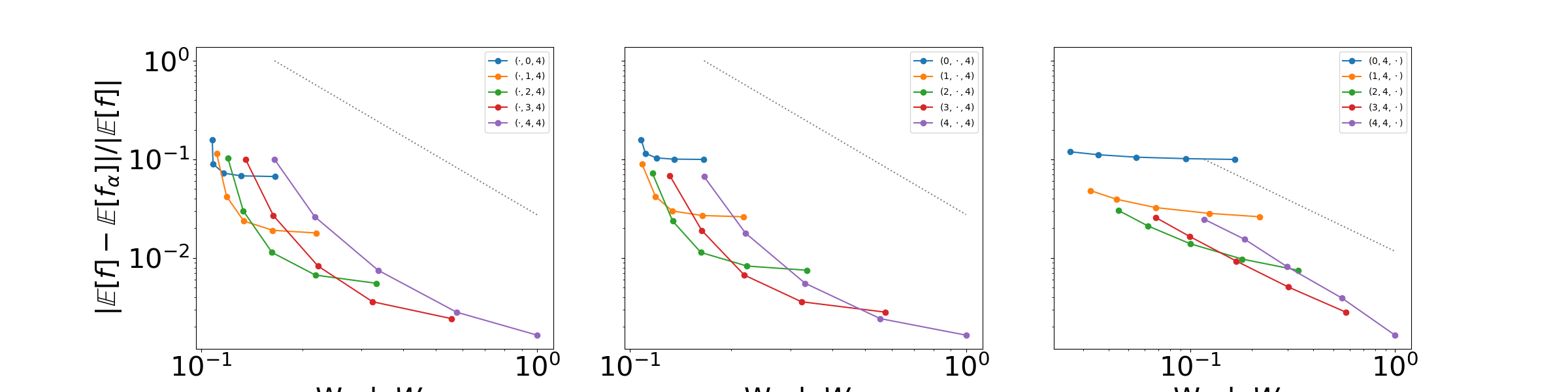
The above figure depicts the changes induced in the error of the mean of the QoI, i.e. $\mathbb{E}[f_\ai]$, as the mesh and temporal discretizations are changed. The legend labels denote the mesh discretization parameter values $(\alpha_1,\alpha_2,\alpha_3)$ used to solve the advection diffusion equation. Numeric values represent discretization parameters that are held fixed while the symbol $\cdot$ denotes that the corresponding parameter is varying. The reference solution is obtained using the model indexed by $(6,6,6)$.

The dashed lines represent the theoretical rates of the convergence of the deterministic error when refining $h_1$ (left), $h_2$ (middle), and $\Delta t$ (right). The error decreases quadratically with both $h_1$ and $h_2$ and linearly with $\Delta t$ until a saturation point is reached. These saturation points occur when the error induced by a coarse resolution in one mesh parameter dominates the others. For example the left plot shows that when refining $h_1$ the final error in $\mathbb{E}[f]$ is dictated by the error induced by using the mesh size $h_2$, provided $\Delta t$ is small enough. Similarly the right plot shows, that for fixed $h_2$, the highest accuracy that can be obtained by refining $\Delta t$ is dependent on the resolution of $h_1$.

Note the expectations computed in the tutorial is estimated using the same 10 samples for all model resolutions. This allows the error in the statistical estimate induced by small numbers of samples to be ignored. The effect of sample size on Monte Carlo estimates of expectations is covered in sphx_glr_auto_tutorials_multi_fidelity_plot_monte_carlo.py.

References

NTWSIAMNA2008

Nobile F, Tempone R, Webster CG. A Sparse Grid Stochastic Collocation Method for Partial Differential Equations with Random Input Data. SIAM Journal on Numerical Analysis 2008;46(5):2309–2345.