Note
Click here to download the full example code
Monte Carlo Quadrature
This tutorial describes how to use Monte Carlo sampling to compute the expectations of the output of an model. The following tutorials on multi-fidelity Monate Carlo methods assume the reader has understanding of the material presented here.
We can approximate th integral \(Q_\alpha\) using Monte Carlo quadrature by drawing \(N\) random samples of \(\rv\) from \(\pdf\) and evaluating the function at each of these samples to obtain the data pairs \(\{(\rv^{(n)},f^{(n)}_\alpha)\}_{n=1}^N\), where \(f^{(n)}_\alpha=f_\alpha(\rv^{(n)})\)
The mean squared error (MSE) of this estimator can be expressed as
Here we used that \(Q_{\alpha,N}\) is an unbiased estimator, i.e. \(\mean{Q_{\alpha,N}}=\mean{Q}\) so the third term on the second line is zero. Now using
yields
From this expression we can see that the MSE can be decomposed into two terms; a so called stochastic error (I) and a deterministic bias (II). The first term is the variance of the Monte Carlo estimator which comes from using a finite number of samples. The second term is due to using an approximation of \(f\). These two errors should be balanced, however in the vast majority of all MC analyses a single model \(f_\alpha\) is used and the choice of \(\alpha\), e.g. mesh resolution, is made a priori without much concern for the balancing bias and variance.
Given a fixed \(\alpha\) the modelers only recourse to reducing the MSE is to reduce the variance of the estimator. In the following we plot the variance of the MC estimate of a simple algebraic function \(f_1\) which belongs to an ensemble of models
where \(\rv_1,\rv_2\sim\mathcal{U}(-1,1)\) and all \(A\) and \(\theta\) coefficients are real. We choose to set \(A=\sqrt{11}\), \(A_1=\sqrt{7}\) and \(A_2=\sqrt{3}\) to obtain unitary variance for each model. The parameters \(s_1,s_2\) control the bias between the models. Here we set \(s_1=1/10,s_2=1/5\). Similarly we can change the correlation between the models in a systematic way (by varying \(\theta_1\). We will levarage this later in the tutorial.
Lets setup the problem
import pyapprox as pya
import numpy as np
import matplotlib.pyplot as plt
from pyapprox.tests.test_control_variate_monte_carlo import TunableModelEnsemble
from scipy.stats import uniform

np.random.seed(1)
univariate_variables = [uniform(-1,2),uniform(-1,2)]
variable = pya.IndependentMultivariateRandomVariable(univariate_variables)
print(variable)
shifts=[.1,.2]
model = TunableModelEnsemble(np.pi/2*.95,shifts=shifts)
Out:
I.I.D. Variable
Number of variables: 2
Unique variables and global id:
    uniform(loc=-1,scale=2): z0, z1
Now let us compute the mean of \(f_1\) using Monte Carlo
nsamples = int(1e3)
samples = pya.generate_independent_random_samples(
    variable,nsamples)
values = model.m1(samples)
pya.print_statistics(samples,values)
Out:
                z0           z1           y0
count  1000.000000  1000.000000  1000.000000
mean      0.001209     0.036225     0.159514
std       0.577001     0.586788     1.026603
min      -0.999771    -0.998471    -2.522199
25%      -0.496131    -0.491685    -0.212117
50%       0.015002     0.067357     0.105057
75%       0.501343     0.560416     0.588887
max       0.994646     0.997041     2.854412
We can compute the exact mean using sympy and compute the MC MSE
import sympy as sp
z1,z2 = sp.Symbol('z1'),sp.Symbol('z2')
ranges = [-1,1,-1,1]
integrand_f1=model.A1*(sp.cos(model.theta1)*z1**3+sp.sin(model.theta1)*z2**3)+shifts[0]*0.25
exact_integral_f1 = float(
    sp.integrate(integrand_f1,(z1,ranges[0],ranges[1]),(z2,ranges[2],ranges[3])))

print('MC difference squared =',(values.mean()-exact_integral_f1)**2)
Out:
MC difference squared = 0.0035419268772882277
Now let us compute the MSE for different sample sets of the same size for \(N=100,1000\) and plot the distribution of the MC estimator \(Q_{\alpha,N}\)
ntrials=1000
means = np.empty((ntrials,2))
for ii in range(ntrials):
    samples = pya.generate_independent_random_samples(
        variable,nsamples)
    values = model.m1(samples)
    means[ii] = values[:100].mean(),values.mean()
fig,ax = plt.subplots()
textstr = '\n'.join([r'$\mathbb{E}[Q_{1,100}]=\mathrm{%.2e}$'%means[:,0].mean(),
                     r'$\mathbb{V}[Q_{1,100}]=\mathrm{%.2e}$'%means[:,0].var(),
                     r'$\mathbb{E}[Q_{1,1000}]=\mathrm{%.2e}$'%means[:,1].mean(),
                     r'$\mathbb{V}[Q_{1,1000}]=\mathrm{%.2e}$'%means[:,1].var()])
ax.hist(means[:,0],bins=ntrials//100,density=True)
ax.hist(means[:,1],bins=ntrials//100,density=True,alpha=0.5)
ax.axvline(x=shifts[0],c='r',label=r'$\mathbb{E}[Q_1]$')
ax.axvline(x=0,c='k',label=r'$\mathbb{E}[Q_0]$')
props = {'boxstyle':'round','facecolor':'white','alpha':1}
ax.text(0.65,0.8,textstr,transform=ax.transAxes,bbox=props)
ax.set_xlabel(r'$\mathbb{E}[Q_N]$')
ax.set_ylabel(r'$\mathbb{P}(\mathbb{E}[Q_N])$')
_ = ax.legend(loc='upper left')
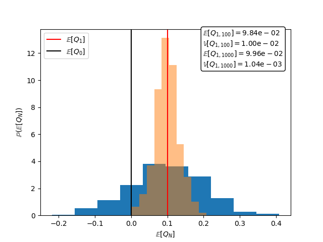
The numerical results match our theory. Specifically the estimator is unbiased( i.e. mean zero, and the variance of the estimator is \(\var{Q_{0,N}}=\var{Q_{0}}/N=1/N\).
The variance of the estimator can be driven to zero by increasing the number of samples \(N\). However when the variance becomes less than the bias, i.e. \(\left(\mean{Q_{\alpha}-Q}\right)^2>\var{Q_{\alpha}}/N\), then the MSE will not decrease and any further samples used to reduce the variance are wasted.
Let our true model be \(f_0\) above. The following code compues the bias induced by using \(f_\alpha=f_1\) and also plots the contours of \(f_0(\rv)-f_1(\rv)\).
integrand_f0 = model.A0*(sp.cos(model.theta0)*z1**5+
                         sp.sin(model.theta0)*z2**5)*0.25
exact_integral_f0 = float(
    sp.integrate(integrand_f0,(z1,ranges[0],ranges[1]),(z2,ranges[2],ranges[3])))
bias = (exact_integral_f0-exact_integral_f1)**2
print('MC f1 bias =',bias)
print('MC f1 variance =',means.var())
print('MC f1 MSE =',bias+means.var())

fig,ax = plt.subplots()
X,Y,Z = pya.get_meshgrid_function_data(
    lambda z: model.m0(z)-model.m1(z),[-1,1,-1,1],50)
cset = ax.contourf(X, Y, Z, levels=np.linspace(Z.min(),Z.max(),20))
_ = plt.colorbar(cset,ax=ax)
#plt.show()
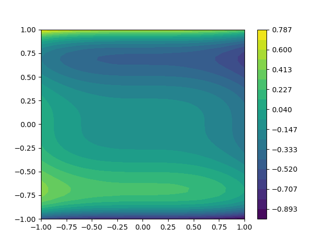
Out:
MC f1 bias = 0.010000000000000018
MC f1 variance = 0.005522183703329499
MC f1 MSE = 0.015522183703329516
As \(N\to\infty\) the MSE will only converge to the bias (\(s_1\)). Try this by increasing \(\texttt{nsamples}\).
We can produced unbiased estimators using the high fidelity model. However if this high-fidelity model is more expensive then this comes at the cost of the estimator having larger variance. To see this the following plots the distribution of the MC estimators using 100 samples of the \(f_1\) and 10 samples of \(f_0\). The cost of constructing these estimators would be equivalent if the high-fidelity model is 10 times more expensive than the low-fidelity model.
ntrials=1000
m0_means = np.empty((ntrials,1))
for ii in range(ntrials):
    samples = pya.generate_independent_random_samples(
        variable,nsamples)
    values = model.m0(samples)
    m0_means[ii] = values[:10].mean()

fig,ax = plt.subplots()
textstr = '\n'.join([r'$\mathbb{E}[Q_{1,100}]=\mathrm{%.2e}$'%means[:,0].mean(),
                     r'$\mathbb{V}[Q_{1,100}]=\mathrm{%.2e}$'%means[:,0].var(),
                     r'$\mathbb{E}[Q_{0,10}]=\mathrm{%.2e}$'%m0_means[:,0].mean(),
                     r'$\mathbb{V}[Q_{0,10}]=\mathrm{%.2e}$'%m0_means[:,0].var()])
ax.hist(means[:,0],bins=ntrials//100,density=True)
ax.hist(m0_means[:,0],bins=ntrials//100,density=True,alpha=0.5)
ax.axvline(x=shifts[0],c='r',label=r'$\mathbb{E}[Q_1]$')
ax.axvline(x=0,c='k',label=r'$\mathbb{E}[Q_0]$')
props = {'boxstyle':'round','facecolor':'white','alpha':1}
ax.text(0.65,0.8,textstr,transform=ax.transAxes,bbox=props)
ax.set_xlabel(r'$\mathbb{E}[Q_N]$')
ax.set_ylabel(r'$\mathbb{P}(\mathbb{E}[Q_N])$')
_ = ax.legend(loc='upper left')
#plt.show()
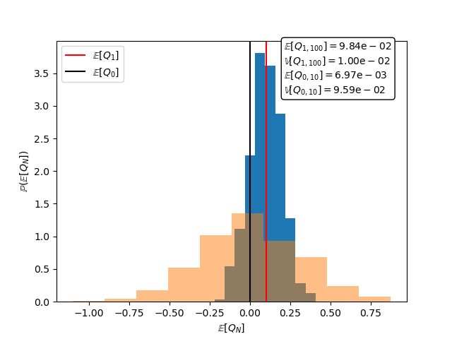
In a series of tutorials starting with Control Variate Monte Carlo we show how to produce an unbiased estimator with small variance using both these models.
Total running time of the script: ( 0 minutes 1.132 seconds)