Bayesian Inference

This tutorial describes how to use Bayesian inference condition estimates of uncertainty on observational data.

Background

When observational data are available, that data should be used to inform prior assumptions of model uncertainties. This so-called inverse problem that seeks to estimate uncertain parameters from measurements or observations is usually ill-posed. Many different realizations of parameter values may be consistent with the data. The lack of a unique solution can be due to the non-convexity of the parameter-to-QoI map, lack of data, and model structure and measurement errors.

Deterministic model calibration is an inverse problem that seeks to find a single parameter set that minimizes the misfit between the measurements and model predictions. A unique solution is found by simultaneously minimising the misfit and a regularization term which penalises certain characteristics of the model parameters.

In the presence of uncertainty we typically do not want a single optimal solution, but rather a probabilistic description of the extent to which different realizations of parameters are consistent with the observations. Bayesian inference~cite{Kaipo_S_book_2005} can be used to define a posterior density for the model parameters \(\rv\) given observational data \(\V{y}=(y_1,\ldots,y_{n_y})\):

Bayes Rule

Given a model \(\mathcal{M}(\rv)\) parameterized by a set of parameters \(\rv\), our goal is to infer the parameter \(\rv\) from data \(d\).

Bayes Theorem describes the probability of the parameters \(\rv\) conditioned on the data \(d\) is proportional to the conditional probability of observing the data given the parameters multiplied by the probability of observing the data, that is

\[\begin{split}\pi (\rv\mid d)&=\frac{\pi (d\mid \rv)\,\pi (\rv)}{\pi(d)}\\ &=\frac{\pi (d\mid \rv)\,\pi (\rv)}{\int_{\mathbb{R}^d} \pi (d\mid \rv)\,\pi (\rv)\,d\rv}\end{split}\]

The density \(\pi (\rv\mid d)\) is referred to as the posterior density.

\[\pi_{\text{post}}(\rv)=\pi_\text(\rv\mid\V{y})=\frac{\pi(\V{y}|\rv)\pi(\rv)}{\int_{\rvdom} \pi(\V{y}|\rv)\pi(\rv)d\rv}\]

Prior

To find the posterior density we must first quantify our prior belief of the possible values of the parameter that can give the data. We do this by specifying the probability of observing the parameter independently of observing the data.

Here we specify the prior distribution to be Normally distributed, e.g

\[\pi\sim N(m_\text{prior},\Sigma_\text{prior})\]

Likelihood

Next we must specify the likelihood \(\pi(d\mid \rv)\) of observing the data given a realizations of the parameter \(\rv\) The likelihood answers the question: what is the distribution of the data assuming that \(\rv\) are the exact parameters?

The form of the likelihood is derived from an assumed relationship between the model and the data.

It is often assumed that

\[d=\mathcal{M}(\rv)+\eta\]

where \(\eta\sim N(0,\Sigma_\text{noise})\) is normally distributed noise with zero mean and covariance \(\Sigma_\text{noise}\).

In this case the likelihood is

\[\pi(d|\rv)=\frac{1}{\sqrt {(2\pi )^{k}|{\boldsymbol {\Sigma_\text{noise} }}}|}\exp \left(-{\frac {1}{2}}(\mathcal{M}(\rv)-d)^{\mathrm {T} }{\boldsymbol {\Sigma_\text{noise} }}^{-1}(\mathcal{M}(\rv)-d)\right)\]

where \(|\Sigma_\text{noise}|=\det \Sigma_\text{noise}\) is the determinant of \(\Sigma_\text{noise}\)

Exact Linear-Gaussian Inference

In the following we will generate data at a truth parameter \(\rv_\text{truth}\) and use Bayesian inference to estimate the probability of any model parameter \(\rv\) conditioned on the observations we generated. Firstly assume \(\mathcal{M}\) is a linear model, i.e.

\[\mathcal{M}(\rv)=A\rv+b,\]

and as above assume that

\[d=\mathcal{M}(\rv)+\eta\]

Now define the prior probability of the parameters to be

\[\pi(\rv)\sim N(m_\text{prior},\Sigma_\text{prior})\]

Under these assumptions, the marginal density (integrating over the prior of \(\rv\)) of the data and parameters is

\[\pi(d)\sim N(m_\text{noise}+Am_\text{prior},\Sigma_\text{noise}+ A\Sigma_\text{prior} A^T)=N(m_\text{data},\Sigma_\text{data})\]

and the joint density of the parameters and data is

\[\pi(\rv,d)\sim N(m_\text{joint},\Sigma_\text{joint})\]

where

\[\begin{split}\boldsymbol m_\text{joint}=\begin{bmatrix} \boldsymbol m_\text{prior} \\ \boldsymbol m_\text{data}\end{bmatrix},\quad \boldsymbol \Sigma_\text{joint}=\begin{bmatrix} \boldsymbol\Sigma_\text{prior} & \boldsymbol\Sigma_\text{prior,data} \\ \boldsymbol\Sigma_\text{prior,data} & \boldsymbol\Sigma_\text{data}\end{bmatrix}\end{split}\]

and

\[\Sigma_\text{prior,data}=A\Sigma_\text{prior}\]

is the covariance between the parameters and data.

Now let us setup this problem in Python

import numpy as np
import pyapprox as pya
import matplotlib.pyplot as plt
from functools import partial
import matplotlib as mpl
np.random.seed(1)

A = np.array([[.5]]); b = 0.0
# define the prior
prior_covariance=np.atleast_2d(1.0)
prior = pya.NormalDensity(0.,prior_covariance)
# define the noise
noise_covariance=np.atleast_2d(0.1)
noise = pya.NormalDensity(0,noise_covariance)
# compute the covariance between the prior and data
C_12 = np.dot(A,prior_covariance)
# define the data marginal distribution
data_covariance = noise_covariance+np.dot(C_12,A.T)
data  = pya.NormalDensity(np.dot(A,prior.mean)+b,
                            data_covariance)
# define the covariance of the joint distribution of the prior and data
def form_normal_joint_covariance(C_11, C_22, C_12):
    num_vars1=C_11.shape[0]
    num_vars2=C_22.shape[0]
    joint_covariance=np.empty((num_vars1+num_vars2,num_vars1+num_vars2))
    joint_covariance[:num_vars1,:num_vars1]=C_11
    joint_covariance[num_vars1:,num_vars1:]=C_22
    joint_covariance[:num_vars1,num_vars1:]=C_12
    joint_covariance[num_vars1:,:num_vars1]=C_12
    return joint_covariance

joint_mean = np.hstack((prior.mean,data.mean))
joint_covariance = form_normal_joint_covariance(
    prior_covariance, data_covariance, C_12)
joint = pya.NormalDensity(joint_mean,joint_covariance)

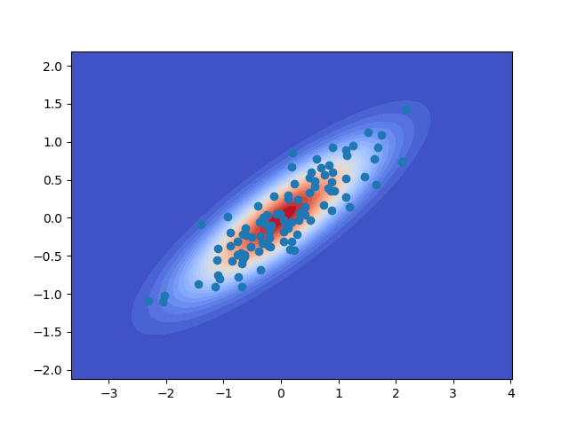
Now we can plot the joint distribution and some samples from that distribution and print the sample covariance of the joint distribution

num_samples=10000
theta_samples = prior.generate_samples(num_samples)
noise_samples = noise.generate_samples(num_samples)
data_samples = np.dot(A,theta_samples) + b +  noise_samples
plot_limits = [theta_samples.min(),theta_samples.max(),
               data_samples.min(),data_samples.max()]
fig,ax = plt.subplots(1,1)
joint.plot_density(plot_limits=plot_limits,ax=ax)
_ = plt.plot(theta_samples[0,:100],data_samples[0,:100],'o')

Out:

/Users/jdjakem/software/pyapprox/pyapprox/visualization.py:279: UserWarning: The following kwargs were not used by contour: 'zdir', 'offset'
  cmap=cmap, zorder=zorder)

Conditional probability of multivariate Gaussians

For multivariate Gaussians the dsitribution of \(x\) conditional on observing the data \(d^\star=d_\text{truth}+\eta^\star\), \(\pi(x\mid d=d^\star)\sim N(m_\text{post},\Sigma_\text{post})\) is a multivariate Gaussian with mean and covariance

\[\begin{split}\boldsymbol{m}_\text{post}&=\boldsymbol m_\text{prior} + \boldsymbol\Sigma_\text{prior,data} \boldsymbol\Sigma_{data}^{-1}\left( \mathbf{d}^\star - \boldsymbol m_\text{data}\right),\\ \boldsymbol \Sigma_\text{post}&=\boldsymbol \Sigma_\text{prior}-\boldsymbol \Sigma_\text{prior,data}\boldsymbol\Sigma_\text{data}^{-1}\boldsymbol\Sigma_\text{data,prior}^T.\end{split}\]

where \(\eta^\star\) is a random sample from the noise variable \(\eta\). In the case of one parameter and one QoI we have

\[\pi(x\mid d=d^\star) \sim\ N\left(m_\text{prior}+\frac{\sigma_\text{prior}}{\sigma_\text{data}}\rho( d^\star - m_\text{data}),\, (1-\rho^2)\sigma_\text{prior}^2\right).\]

where the correlation coefficient between the parameter and data is

Lets use this formula to update the prior when one data \(d^\star\) becomes available.

def condition_normal_on_data(mean, covariance, fixed_indices, values):
    indices = set(np.arange(mean.shape[0]))
    ind_remain = list(indices.difference(set(fixed_indices)))
    new_mean = mean[ind_remain]
    diff = values - mean[fixed_indices]
    sigma_11 = np.array(covariance[ind_remain, ind_remain], ndmin=2)
    sigma_12 = np.array(covariance[ind_remain, fixed_indices], ndmin=2)
    sigma_22 = np.array(covariance[fixed_indices, fixed_indices], ndmin=2)
    update = np.dot(sigma_12, np.linalg.solve(sigma_22, diff)).flatten()
    new_mean = new_mean + update
    new_cov = sigma_11-np.dot(sigma_12, np.linalg.solve(sigma_22, sigma_12.T))
    return new_mean, new_cov

x_truth=0.2;
data_obs = np.dot(A,x_truth)+b+noise.generate_samples(1)

new_mean, new_cov = condition_normal_on_data(
    joint_mean, joint_covariance,[1],data_obs)
posterior = pya.NormalDensity(new_mean,new_cov)

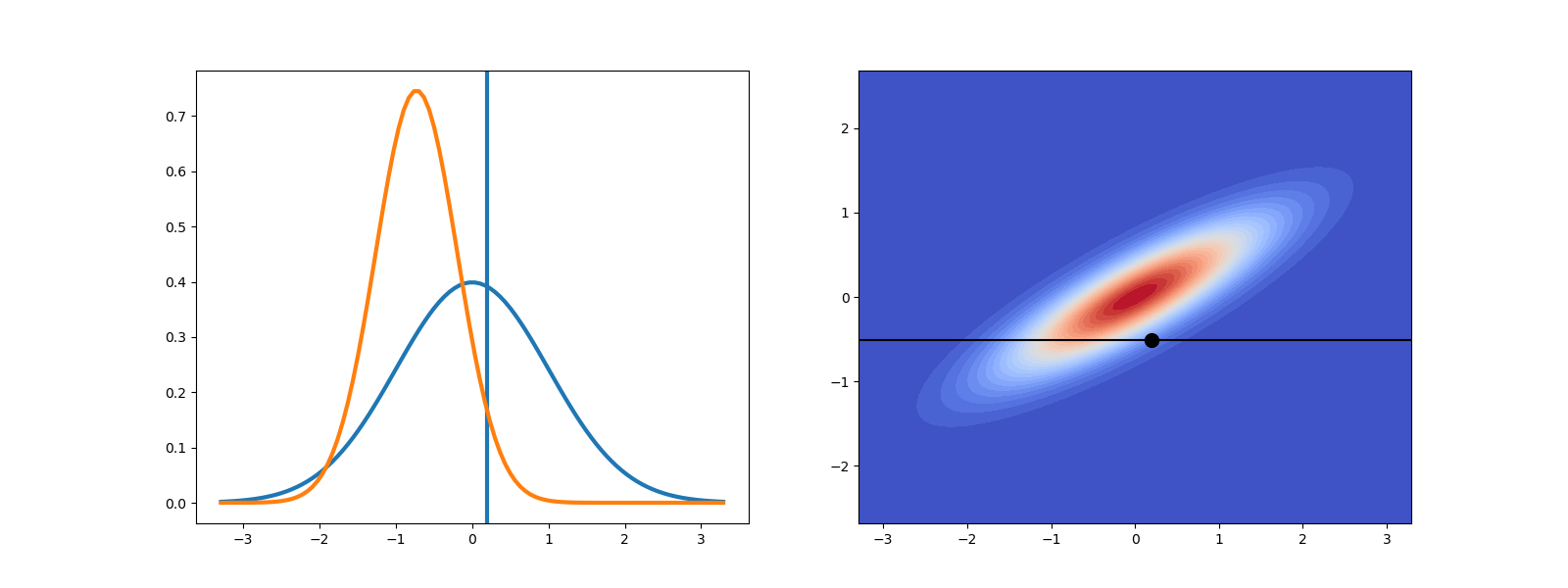
Now lets plot the prior and posterior of the parameters as well as the joint distribution and the data.

f, axs = plt.subplots(1,2,figsize=(16,6))
prior.plot_density(label='prior',ax=axs[0])
axs[0].axvline(x=x_truth,lw=3,label=r'$x_\text{truth}$')
posterior.plot_density(plot_limits=prior.plot_limits, ls='-',label='posterior',ax=axs[0])
colorbar_lims=None#[0,1.5]
joint.plot_density(ax=axs[1],colorbar_lims=colorbar_lims)
axhline=axs[1].axhline(y=data_obs,color='k')
axplot=axs[1].plot(x_truth,data_obs,'ok',ms=10)

Out:

/Users/jdjakem/software/pyapprox/pyapprox/visualization.py:279: UserWarning: The following kwargs were not used by contour: 'zdir', 'offset'
  cmap=cmap, zorder=zorder)

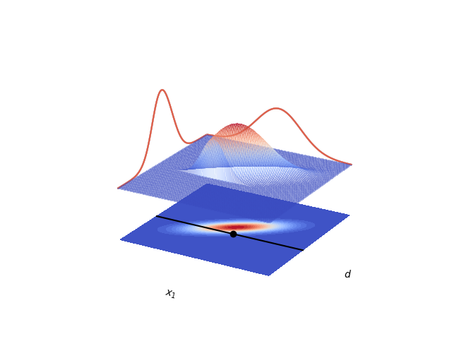
Lets also plot the joint distribution and marginals in a 3d plot

def data_obs_limit_state(samples, vals, data_obs):
    vals = np.ones((samples.shape[1]),float)
    I = np.where(samples[1,:]<=data_obs[0,0])[0]
    return I, 0.

num_pts_1d=100
limit_state = partial(data_obs_limit_state,data_obs=data_obs)
X,Y,Z=pya.get_meshgrid_function_data(
    joint.pdf, joint.plot_limits, num_pts_1d, qoi=0)
offset=-(Z.max()-Z.min())
samples = np.array([[x_truth,data_obs[0,0],offset]]).T
ax = pya.create_3d_axis()
pya.plot_surface(X,Y,Z,ax,axis_labels=[r'$x_1$',r'$d$',''],
                 limit_state=limit_state,
                 alpha=0.3,cmap=mpl.cm.coolwarm,zorder=3,plot_axes=False)
num_contour_levels=30;
cset = pya.plot_contours(X,Y,Z,ax,num_contour_levels=num_contour_levels,
                    offset=offset,cmap=mpl.cm.coolwarm,zorder=-1)
Z_prior=prior.pdf(X.flatten()).reshape(X.shape[0],X.shape[1])
ax.contour(X, Y, Z_prior, zdir='y', offset=Y.max(), cmap=mpl.cm.coolwarm)
Z_data=data.pdf(Y.flatten()).reshape(Y.shape[0],Y.shape[1])
ax.contour(X, Y, Z_data, zdir='x', offset=X.min(), cmap=mpl.cm.coolwarm)
ax.set_zlim(Z.min()+offset, max(Z_prior.max(),Z_data.max()))
x = np.linspace(X.min(),X.max(),num_pts_1d);
y = data_obs[0,0]*np.ones(num_pts_1d)
z = offset*np.ones(num_pts_1d)
ax.plot(x,y,z,zorder=100,color='k')
_ = ax.plot([x_truth],[data_obs[0,0]],[offset],zorder=100,color='k',marker='o')

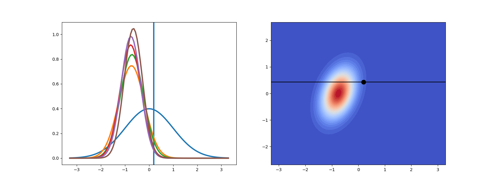
Now lets assume another piece of observational data becomes available we can use the posterior as a new prior.

num_obs=5
posteriors = [None]*num_obs
posteriors[0]=posterior
for ii in range(1,num_obs):
    new_prior=posteriors[ii-1]
    data_obs = np.dot(A,x_truth)+b+noise.generate_samples(1)
    C_12 = np.dot(A,new_prior.covariance)
    new_joint_covariance = form_normal_joint_covariance(
        new_prior.covariance, data.covariance, C_12)
    new_joint = pya.NormalDensity(np.hstack((new_prior.mean,data.mean)),
                              new_joint_covariance)
    new_mean, new_cov = condition_normal_on_data(
        new_joint.mean, new_joint.covariance,
        np.arange(new_prior.num_vars(),new_prior.num_vars()+data.num_vars()),
       data_obs)
    posteriors[ii] = pya.NormalDensity(new_mean,new_cov)

And now lets again plot the joint density before the last data was added and final posterior and the intermediate priors.

f, axs = plt.subplots(1,2,figsize=(16,6))
prior.plot_density(label='prior',ax=axs[0])
axs[0].axvline(x=x_truth,lw=3,label=r'$x_\text{truth}$')
for ii in range(num_obs):
    posteriors[ii].plot_density(plot_limits=prior.plot_limits, ls='-',label='posterior',ax=axs[0])

colorbar_lims=None
new_joint.plot_density(ax=axs[1],colorbar_lims=colorbar_lims,
                       plot_limits=joint.plot_limits)
axhline=axs[1].axhline(y=data_obs,color='k')
axplot=axs[1].plot(x_truth,data_obs,'ok',ms=10)

Out:

/Users/jdjakem/software/pyapprox/pyapprox/visualization.py:279: UserWarning: The following kwargs were not used by contour: 'zdir', 'offset'
  cmap=cmap, zorder=zorder)

As you can see the variance of the joint density decreases as more data is added. The posterior variance also decreases and the posterior will converge to a Dirac-delta function as the number of observations tends to infinity. Currently the mean of the posterior is not near the true parameter value (the horizontal line). Try increasing num_obs1 to see what happens.

Inexact Inference using Markov Chain Monte Carlo

When using non-linear or non-Gaussian priors, a functional representation of the posterior distribution \(\pi_\text{post}\) cannot be computed analytically. Instead the the posterior is characterized by samples drawn from the posterior using Markov-chain Monte Carlo (MCMC) sampling methods.

Lets consider non-linear model with two uncertain parameters with independent uniform priors on [-2,2] and the negative log likelihood function

\[-\log\left(\pi(d\mid\rv)\right)=\frac{1}{10}\rv_1^4 + \frac{1}{2}(2\rv_2-\rv_1^2)^2\]

We can sample the posterior using Sequential Markov Chain Monte Carlo using the following code.

import matplotlib
import matplotlib.pyplot as plt
import numpy as np
import pyapprox as pya
from scipy.stats import uniform
from pyapprox.bayesian_inference.tests.test_markov_chain_monte_carlo import \
    ExponentialQuarticLogLikelihoodModel
from pyapprox.bayesian_inference.markov_chain_monte_carlo import \
    run_bayesian_inference_gaussian_error_model, PYMC3LogLikeWrapper
np.random.seed(1)

univariate_variables = [uniform(-2,4),uniform(-2,4)]
plot_range = np.asarray([-1,1,-1,1])*2
variables = pya.IndependentMultivariateRandomVariable(univariate_variables)

loglike = ExponentialQuarticLogLikelihoodModel()
loglike = PYMC3LogLikeWrapper(loglike)

# number of draws from the distribution
ndraws = 500
# number of "burn-in points" (which we'll discard)
nburn = min(1000,int(ndraws*0.1))
# number of parallel chains
njobs=1
samples, effective_sample_size, map_sample = \
    run_bayesian_inference_gaussian_error_model(
        loglike,variables,ndraws,nburn,njobs,
        algorithm='smc',get_map=True,print_summary=True)

print('MAP sample',map_sample.squeeze())

Out:

  0%|          | 0/5000 [00:00<?, ?it/s]
logp = -2.7726:   0%|          | 0/5000 [00:00<?, ?it/s]
logp = -2.7726:   0%|          | 10/5000 [00:00<00:00, 7188.18it/s]
logp = -2.7726:   0%|          | 20/5000 [00:00<00:00, 8702.78it/s]
logp = -2.7726:   1%|          | 30/5000 [00:00<00:00, 9241.95it/s]
logp = -2.7726:   1%|          | 40/5000 [00:00<00:00, 9617.76it/s]
logp = -2.7726:   1%|1         | 50/5000 [00:00<00:00, 9165.47it/s]
logp = -2.7726:   1%|1         | 60/5000 [00:00<00:00, 9384.98it/s]
logp = -2.7726: 100%|##########| 62/62 [00:00<00:00, 9267.53it/s]
could not print summary. likely issue with theano
could not compute ess. likely issue with theano
could not compute ess. likely issue with theano
MAP sample [ 1.23767663e-11 -7.43454187e-11]

The NUTS sampler offerred by PyMC3 can also be used by specifying algorithm=’nuts’. This sampler requires gradients of the likelihood function which if not provided will be computed using finite difference.

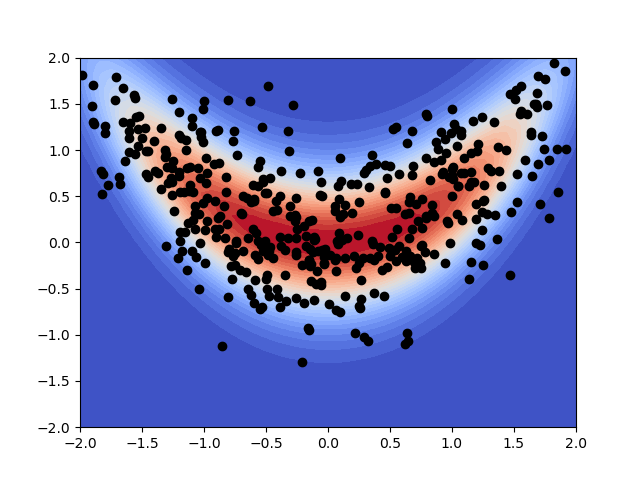
Lets plot the posterior distribution and the MCMC samples. First we must compute the evidence

def unnormalized_posterior(x):
    vals = np.exp(loglike.loglike(x))
    rvs = variables.all_variables()
    for ii in range(variables.num_vars()):
        vals[:,0] *= rvs[ii].pdf(x[ii,:])
    return vals

def univariate_quadrature_rule(n):
    x,w = pya.gauss_jacobi_pts_wts_1D(n,0,0)
    x*=2
    return x,w
x,w = pya.get_tensor_product_quadrature_rule(
    100,variables.num_vars(),univariate_quadrature_rule)
evidence = unnormalized_posterior(x)[:,0].dot(w)
print('evidence',evidence)

plt.figure()
X,Y,Z = pya.get_meshgrid_function_data(
    lambda x: unnormalized_posterior(x)/evidence, plot_range, 50)
plt.contourf(
    X, Y, Z, levels=np.linspace(Z.min(),Z.max(),30),
    cmap=matplotlib.cm.coolwarm)
plt.plot(samples[0,:],samples[1,:],'ko')
plt.show()

Out:

evidence 0.014953532968320147

Now lets compute the mean of the posterior using a highly accurate quadrature rule and compars this to the mean estimated using MCMC samples.

exact_mean = ((x*unnormalized_posterior(x)[:,0]).dot(w)/evidence)
#print(exact_mean)
print('mcmc mean',samples.mean(axis=1))
print('exact mean',exact_mean.squeeze())

Out:

mcmc mean [-0.04713958  0.42756304]
exact mean [-1.23718604e-16  4.33326051e-01]