Gaussian Networks

This tutorial describes how to perform efficient inference on a network of Gaussian-linear models using Bayesian networks, often referred to as Gaussian networks. Bayesian networks can be constructed to provide a compact representation of joint distribution, which can be used to marginalize out variables and condition on observational data without the need to construct a full representation of the joint density over all variables.

Directed Acyclic Graphs

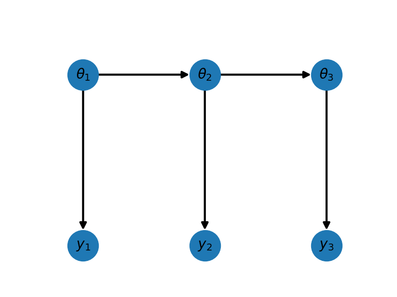
A Bayesian network (BN) structure is a directed acyclic graphs (DAG) whose nodes represent random variables and whose edges represent probabilistic relationships between them. The graph can be represented by a tuple of vertices (or nodes) and edges $\mathcal{G} = \left( \mathbf{V}, \mathbf{E} \right)$. A node $\theta_{j} \in \mathbf{V}$ is a parent of a random variable $\theta_{i} \in \mathbf{V}$ if there is a directed edge $[\theta_{j} \to \theta_{i}] \in \mathbf{E}$. The set of parents of random variable $\theta_{i}$ is denoted by $\theta_{\mathrm{pa}(i)}$.

Lets import some necessary modules and then construct a DAG consisting of 3 groups of variables.

import numpy as np
from scipy import stats
import pyapprox as pya
from pyapprox.gaussian_network import *
import copy
from pyapprox.configure_plots import *
np.random.seed(1)

nnodes=3
fig,ax=plt.subplots(1,1,figsize=(8,3))
_=plot_hierarchical_network(nnodes,ax)
fig.tight_layout()

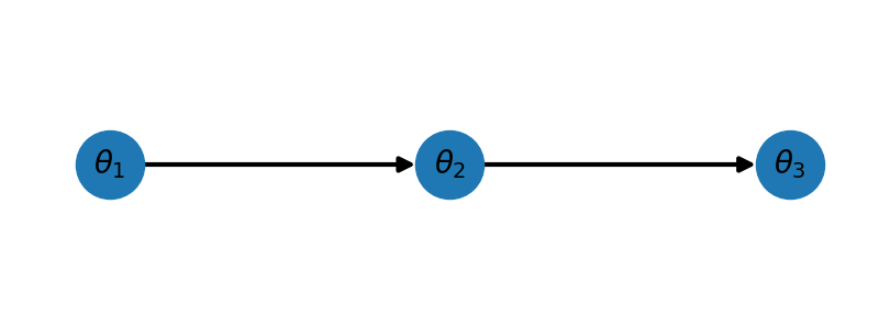
For this network we have $\mathrm{pa}(\theta_1)=\emptyset,\;\mathrm{pa}(\theta_2)=\{\theta_1\},\;\mathrm{pa}(\theta_3)=\{\theta_2\}$.

Conditional probability distributions

Bayesian networks use onditional probability distributions (CPDs) to encode the relationships between variables of the graph. Let $A,B,C$ denote three random variables. $A$ is conditionally independent of $B$ given $C$ in distribution $\mathbb{P}$, denoted by $A \mathrel{\perp\mspace{-10mu}\perp} B \mid C$, if

$$\mathbb{P}(A = a, B = b \mid C = c) = \mathbb{P}(A = a\mid C=c) \mathbb{P}(B = b \mid C = c).$$

The above graph encodes that $\theta_1\mathrel{\perp\mspace{-10mu}\perp} \theta_3 \mid \theta_2$. CPDs, such as this, can be used to form a compact representation of the joint density between all variables in the graph. Specifically, the joint distribution of the variables can be expressed as a product of the set of conditional probability distributions

$$\mathbb{P}(\theta_{1}, \ldots \theta_{M}) = \prod_{i=1}^M \mathbb{P}(\theta_{i} \mid \theta_{\mathrm{pa}(i)}).$$

For our example we have

$$\mathbb{P}(\theta_1,\theta_2,\theta_3)= \mathbb{P}(\theta_1\mid\mathrm{pa}(\theta_1))\mathbb{P}(\theta_2\mid\mathrm{pa}(\theta_2))\mathbb{P}(\theta_3\mid\mathrm{pa}(\theta_3))=\mathbb{P}(\theta_1)\mathbb{P}(\theta_2\mid \theta_1)\mathbb{P}(\theta_3\mid\theta_2)$$

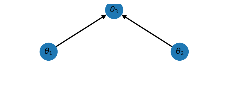
Any Bayesian networks can be made up of three types of structures. The hierarchical (or serial) structure we just plotted and the diverging and peer (or V-) structure.

For the peer network plotted using the code below we have $\mathrm{pa}(\theta_1)=\emptyset,\;\mathrm{pa}(\theta_2)=\emptyset,\;\mathrm{pa}(\theta_3)=\{\theta_1,\theta_2\}$ and

$$\mathbb{P}(\theta_1,\theta_2,\theta_3)= \mathbb{P}(\theta_1\mid\mathrm{pa}(\theta_1))\mathbb{P}(\theta_2\mid\mathrm{pa}(\theta_2))\mathbb{P}(\theta_3\mid\mathrm{pa}(\theta_3))=\mathbb{P}(\theta_1)\mathbb{P}(\theta_2)\mathbb{P}(\theta_3\mid\theta_1,\theta_2)$$

nnodes=3
fig,ax=plt.subplots(1,1,figsize=(8,3))
_=plot_peer_network(nnodes,ax)
fig.tight_layout()

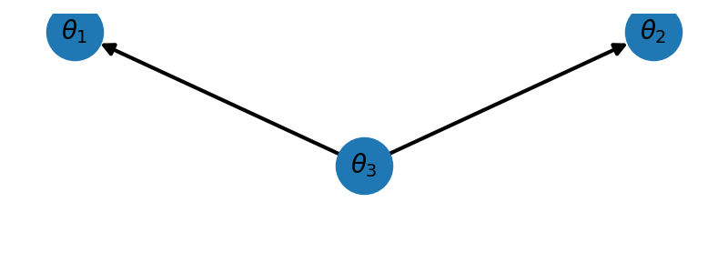
For the diverging network plotted using the code below we have $\mathrm{pa}(\theta_1)=\{\theta_3\},\;\mathrm{pa}(\theta_2)=\{\theta_3\},\;\mathrm{pa}(\theta_3)=\emptyset$ and

$$\mathbb{P}(\theta_1,\theta_2,\theta_3)= \mathbb{P}(\theta_1\mid\mathrm{pa}(\theta_1))\mathbb{P}(\theta_2\mid\mathrm{pa}(\theta_2))\mathbb{P}(\theta_3\mid\mathrm{pa}(\theta_3))=\mathbb{P}(\theta_3)\mathbb{P}(\theta_1\mid \theta_3)\mathbb{P}(\theta_2\mid\theta_3)$$

nnodes=3
fig,ax=plt.subplots(1,1,figsize=(8,3))
_=plot_diverging_network(nnodes,ax)
fig.tight_layout()

For Gaussian networks we assume that the parameters of each node $\theta_i=[\theta_{i,1},\ldots,\theta_{i,P_i}]^T$ are related by

$$\theta_i = \sum_{j\in\mathrm{pa}(i)} A_{ij}\theta_j + b_i + v_i,$$

where $b_i\in\reals^{P_i}$ is a deterministic shift, $v_i$ is a Gaussian noise with mean zero and covariance $\Sigma_{v_i}\in\reals^{P_i\times P_i}$. Consequently, the CPDs take the form

$$\mathbb{P}(\theta_{i} \mid \theta_{\mathrm{pa}(i)}) \sim \mathcal{N}\left(\sum_{j\in\mathrm{pa}(i)} A_{ij}\theta_j + b_i,\Sigma_{vi}\right)$$

which means that $\theta_{i}\sim\mathcal{N}\left(\mu_i,\Sigma_{ii}\right)$ where

$$\mu_i=b_i+A_{ij}\mu_j, \qquad \Sigma_{ii}=\Sigma_{vi}+A_{ij}\Sigma_{jj}A_{ij}^T$$

The Canonical Form

Unless a variable $\theta_i$ is a root node of a network, i.e. $\mathrm{pa}(\theta_i)=\emptyset$ the CPD is in general not Gaussian; for root nodes the CPD is just the density of $\theta_i$. However we can represent the CPDs of no-root nodes and the Gaussian density of root nodes with a consistent reprsentation. Specifically we will use the canonical form of a set of variables $X$

$$\mathcal{\phi}(x;K,h,g) = \exp\left(g+h^T x-\frac{1}{2} x^T K x\right)$$

This canonical form can be used to represent each CPD in a graph such that

$$\mathbb{P}(\theta_1,\ldots,\theta_M) = \prod_{i=1}^M \phi_i$$

For example, the hierarchical structure can be represented by three canonical factors $\phi_1(\theta_1),\phi_2(\theta_1,\theta_2),\phi_3(\theta_2,\theta_3)$ such that

$$\mathbb{P}(\theta_1,\theta_2,\theta_3) = \phi_1(\theta_1)\phi_2(\theta_1,\theta_2)\phi_3(\theta_2,\theta_3)$$

where we have dropped the dependence on $K,h,g$ for convenience. These three factors respectively correspond to the three CPDs $\mathbb{P}(\theta_1),\mathbb{P}(\theta_2\mid\theta_1),\mathbb{P}(\theta_3\mid\theta_2)$

To form the joint density (which we want to avoid in practice) and perform inference and marginalization of a Gaussian graph we must first understand the notion of scope and three basic operations on canonical factors: multiplication, marginalization and conditioning also knows as reduction.

Multiplying Canonical Forms

The scope of canonical forms

The scope of a canonical form $\phi(x)$ is the set of variables $X$ and is denoted $\mathrm{Scope}[\phi]$. Consider the hierarchical structure, just discussed the scope of the 3 factors are

$$\mathrm{Scope}[\phi_1]=\{\theta_1\},\quad\mathrm{Scope}[\phi_2]=\{\theta_1,\theta_2\},\quad\mathrm{Scope}[\phi_3]=\{\theta_2,\theta_3\}.$$

The multiplication of canonical factors with the same scope is simple $X$ is simple

$$\phi_1(X;K_1,h_1,g_1)\phi_2(X;K_2,h_2,g_2)=\phi_1(X;K_1+K_2,h_1+h_2,g_1+g_2).$$

To multiply two canonical forms with different scopes we must extend the scopes to match and then apply the previous formula. This can be done by adding zeros in $K$ and $h$ of the canonical form. For example consider the two canonical factors of the $\theta_1,\theta_2$ with $P_1=1,P_2=1$

$$\begin{split}\phi_2\left(\theta_1,\theta_2;\begin{bmatrix}K_{2,11} & K_{2,12}\\ K_{2,21} & K_{2,22}\end{bmatrix},\begin{bmatrix}h_{2,1}\\ h_{2,2} \end{bmatrix},g_2\right), \phi_3\left(\theta_2,\theta_3;\begin{bmatrix}K_{3,11} & K_{3,12}\\ K_{3,21} & K_{3,22}\end{bmatrix},\begin{bmatrix}h_{2,1}\\ h_{3,2} \end{bmatrix},g_3\right)\end{split}$$

Extending the scope and multiplying proceeds as follows

$$\begin{split}&\phi_2\left(\theta_1,\theta_2,\theta_3;\begin{bmatrix}K_{2,11} & K_{2,12} & 0\\ K_{2,21} & K_{2,22} & 0\\ 0 & 0 & 0\end{bmatrix},\begin{bmatrix}h_{2,1}\\ h_{2,2}\\0 \end{bmatrix},g_2\right)\phi_3\left(\theta_1,\theta_2,\theta_3;\begin{bmatrix}0 & 0 & 0 \\ 0 & K_{3,11} & K_{3,12}\\ 0 &K_{3,21} & K_{3,22}\end{bmatrix},\begin{bmatrix}h_{2,1}\\ h_{3,2} \end{bmatrix},g_3\right)\\=&\phi_{2\times 3}\left(\theta_1,\theta_2,\theta_3;\begin{bmatrix}K_{2,11} & K_{2,12} & 0\\ K_{2,21} & K_{2,22}+K_{3,11} & K_{3,12}\\ 0 & K_{3,21} & K_{3,22}\end{bmatrix},\begin{bmatrix}h_{2,1}\\ h_{2,2}+h_{3,1}\\h_{3,2} \end{bmatrix},g_2+g_3\right)\end{split}$$

The canonical form of a Gaussian distribution

Now we understand how to multiply two factors of different scope we can now discuss how to convert CPDs into canonical factors. The canonical form of a normal distribution with mean $m$ and covariance $C$ has the parameters $K=C^{-1}$, $h = K m$ and

$$g = -\frac{1}{2} m^T h -\frac{1}{2} n\log(2\pi) +\frac{1}{2} \log |K|.$$

The derivation of these expressions is simple and we leave to the reader. The derivation of the canonical form of a linear-Gaussian CPD is more involved however and we derive it here.

The canonical form of a CPD

First we assume that the joint density of two Gaussian variables $\theta_i,\theta_j$ can be represented as the product of two canonical forms referred to as factors. Specifically let $\phi_{i}(\theta_i,\theta_j)$ be the factor representing the CPD $\mathbb{P}(\theta_i\mid\theta_j)$, let $\phi_{j}$ be the canonical form of the Gaussian $\theta_j$, and assume

$$\mathbb{P}(\theta_i,\theta_j)=\mathbb{P}(\theta_i\mid\theta_j)\mathbb{P}(\theta_j)=\phi_{\theta_i}\phi_{\theta_j}$$

Given the linear relationship of the CPD $\theta_i=A_ij\theta_j+v_i$ the inverse of the covariance of the Gaussian joint density $\mathbb{P}(\theta_i,\theta_j)$ is

$$\begin{split}K_{i}&=\begin{bmatrix}\Sigma_{jj} & \Sigma_{jj}A_{ij}^T\\ A_{ij}\Sigma_{jj} & A_{ij}\Sigma_{jj}A_{ij}^T + \Sigma_{vi}\end{bmatrix}^{-1}\\ &=\begin{bmatrix}\Sigma_{jj}^{-1}+ A_{ij}^T\Sigma_{vi}^{-1}A_{ij} & -A_{ij}^T\Sigma_{vi}^{-1}\\ -\Sigma_{vi}^{-1}A_{ij} & \Sigma_{vi}^{-1}\end{bmatrix}\end{split}$$

where the second equality is derived using the matrix inversion lemma. Because $\mathbb{P}(\theta_i)$phi_j` has $K_j=\Sigma_{jj}^{-1}\in\reals^{P_j\times P_j}$. Multiply he two canonical factors, making sure to account for the different scopes we have

$$\begin{split}\begin{bmatrix}\Sigma_{jj}^{-1} & 0 \\ 0 & 0\end{bmatrix}\begin{bmatrix}K_{i11} & K_{i12} \\ K_{i21} & K_{i22}\end{bmatrix}=\begin{bmatrix}\Sigma_{jj}^{-1}+ A_{ij}^T\Sigma_{vi}^{-1}A_{ij} & -A_{ij}^T\Sigma_{vi}^{-1}\\ -\Sigma_{vi}^{-1}A_{ij} & \Sigma_{vi}^{-1}\end{bmatrix}\end{split}$$

Equating terms in the above equation yields

(1) $$K_{i11}=A_{ij}^T\Sigma_{vi}^{-1}A_{ij},\quad K_{i12}=K_{i21}^T=-A_{ij}^T\Sigma_{vi}^{-1},\quad K_{i22}=\Sigma_{vi}^{-1}.$$

A similar procedure can be used to find $h=[(A_{ij}^T\Sigma_{vi}^{-1}b)^T,(\Sigma_{vi}^{-1}b)^T]^T$ and $g$.

Computing the joint density with the canonical forms

We are now in a position to be able to compute the joint density of all the variables in a Gaussian Network. Note that we would never want to do this in practice because it negates the benefit of having the compact representation provided by the Gaussian network.

The following builds a hierarchical network with three ndoes. Each node has $P_i=2$ variables. We set the matrices $A_{ij}=a_{i}jI$ to be a diagonal matrix with the same entries $a_{ij}$ along the diagonal. This means that we are saying that only the $k$-th variable $k=1,\ldots,P_i$ of the $i$-th node is related to the $k$-th variable of the $j$-th node.

nnodes = 3
graph = nx.DiGraph()
prior_covs = [1,2,3]
prior_means = [-1,-2,-3]
cpd_scales  =[0.5,0.4]
node_labels = [f'Node_{ii}' for ii in range(nnodes)]
nparams = np.array([2]*3)
cpd_mats  = [None,cpd_scales[0]*np.eye(nparams[1],nparams[0]),
             cpd_scales[1]*np.eye(nparams[2],nparams[1])]

Now we set up the directed acyclic graph providing the information to construct the CPDs. Specifically we specify the Gaussian distributions of all the root nodes. in this example there is just one root node $\theta_i$. We then specify the parameters of the CPDs for the remaining two nodes. Here we specify the CPD covariance $\Sigma_{vi}$ and shift $b_i$ such that the mean and variance of the paramters matches those specified above. To do this we note that

$$\begin{split}\mean{\theta_2}&=\mean{A_{21}\theta_1+b_2}=A_{21}\mean{\theta_1}+b_2\\ \mean{\theta_3}&=A_{32}\mean{\theta_2}+b_3\end{split}$$

and so set

$$\begin{split}b_2&=\mean{\theta_2}-A_{21}\mean{\theta_1}\\ b_3&=\mean{\theta_3}-A_{32}\mean{\theta_2}.\end{split}$$

Similarly we define the CPD covariance so that the diagonal of the prior covariance matches the values specified

$$\begin{align}\begin{aligned} \var{\theta_2}=\Sigma_{v2}+A_{21}\var{\theta_1}A_{21}^T,\qquad \var{\theta_3}=\Sigma_{32}+A_{32}\var{\theta_2}A_{32}^T\\so\end{aligned}\end{align}$$

$$\Sigma_{21}=\var{\theta_2}-A_{21}\var{\theta_1}A_{21}^T,\qquad \Sigma_{32}=\var{\theta_3}-A_{32}\var{\theta_2}A_{32}^T$$

ii=0
graph.add_node(
    ii,label=node_labels[ii],cpd_cov=prior_covs[ii]*np.eye(nparams[ii]),
    nparams=nparams[ii],cpd_mat=cpd_mats[ii],
    cpd_mean=prior_means[ii]*np.ones((nparams[ii],1)))
for ii in range(1,nnodes):
    cpd_mean = np.ones((nparams[ii],1))*(
        prior_means[ii]-cpd_scales[ii-1]*prior_means[ii-1])
    cpd_cov = np.eye(nparams[ii])*max(
        1e-8,prior_covs[ii]-cpd_scales[ii-1]**2*prior_covs[ii-1])
    graph.add_node(ii,label=node_labels[ii],cpd_cov=cpd_cov,
                   nparams=nparams[ii],cpd_mat=cpd_mats[ii],
                   cpd_mean=cpd_mean)

graph.add_edges_from([(ii,ii+1) for ii in range(nnodes-1)])


network = GaussianNetwork(graph)
network.convert_to_compact_factors()
labels = [l[1] for l in network.graph.nodes.data('label')]
factor_prior = network.factors[0]
for ii in range(1,len(network.factors)):
    factor_prior *= network.factors[ii]
prior_mean,prior_cov = convert_gaussian_from_canonical_form(
    factor_prior.precision_matrix,factor_prior.shift)
print('Prior Mean\n',prior_mean)
print('Prior Covariance\n',prior_cov)

Out:

Prior Mean
 [-1. -1. -2. -2. -3. -3.]
Prior Covariance
 [[1.  0.  0.5 0.  0.2 0. ]
 [0.  1.  0.  0.5 0.  0.2]
 [0.5 0.  2.  0.  0.8 0. ]
 [0.  0.5 0.  2.  0.  0.8]
 [0.2 0.  0.8 0.  3.  0. ]
 [0.  0.2 0.  0.8 0.  3. ]]

We can check the mean and covariance diagonal of the prior match the values we specified

true_prior_mean = np.hstack(
    [[prior_means[ii]]*nparams[ii] for ii in range(nnodes)])
assert np.allclose(true_prior_mean,prior_mean)
true_prior_var = np.hstack(
    [[prior_covs[ii]]*nparams[ii] for ii in range(nnodes)])
assert np.allclose(true_prior_var,np.diag(prior_cov))

If the reader is interested they can also compare the entire prior covariance with

$$\begin{split}\begin{bmatrix}\Sigma_{11} & \Sigma_{11}A_{12}^T & \Sigma_{11}A_{12}^TA_{32}^T \\ A_{21}\Sigma_{11} & \Sigma_{22} & \Sigma_{22}A_{32}^T\\ A_{32}A_{21}\Sigma_{11} & A_{32}\Sigma_{22} & \Sigma_{33}\end{bmatrix}\end{split}$$

Conditioning The Canonical Form

Using the canonical form of these factors we can easily condition them on available data. Given a canonical form over two variables $X,Y$ with

(2) $$\begin{split}K=\begin{bmatrix} K_{XX} & K_{XY}\\ K_{YX} & K_{YY}\end{bmatrix}, \qquad h=\begin{bmatrix}h_{X} \\h_{Y}\end{bmatrix}\end{split}$$

and given data $y$ (also called evidence in the literature) the paramterization of the canonical form of the factor conditioned on the data is simply

(3) $$K^\prime=K_{XX}, \quad h^\prime=h_X-K_{XY}y, \quad g^\prime=g+h_Y^Ty-\frac{1}{2}y^TK_{yy}y$$

Classical inference for linear Gaussian models as a two node network

Gaussian networks enable efficient inference of the unknown variables using observational data. Classical inference for linear-Gaussian models can be represented with a graph consiting of two nodes. First setup a dataless graph of one node

nnodes=1
graph = nx.DiGraph()
ii=0
graph.add_node(
    ii,label=node_labels[ii],cpd_cov=prior_covs[ii]*np.eye(nparams[ii]),
    nparams=nparams[ii],cpd_mat=cpd_mats[ii],
    cpd_mean=prior_means[ii]*np.ones((nparams[ii],1)))

nsamples = [10]
noise_std=[0.01]*nnodes
data_cpd_mats=[np.random.normal(0,1,(nsamples[ii],nparams[ii]))
               for ii in range(nnodes)]
data_cpd_vecs=[np.ones((nsamples[ii],1)) for ii in range(nnodes)]
true_coefs=[np.random.normal(0,np.sqrt(prior_covs[ii]),(nparams[ii],1))
            for ii in range(nnodes)]
noise_covs=[np.eye(nsamples[ii])*noise_std[ii]**2
            for ii in range(nnodes)]

network = GaussianNetwork(graph)

Now lets add data and plot the new graph. Specifically we will add data

$$Y=\Phi\theta_1+b+\epsilon$$

Which has the form of a CPD. Here epsilon is mean zero Gaussian noise with covariance $\Sigma_{\epsilon}=\sigma^2I$.

network.add_data_to_network(data_cpd_mats,data_cpd_vecs,noise_covs)

fig,ax=plt.subplots(1,1,figsize=(8,6))
plot_hierarchical_network_network_with_data(network.graph,ax)

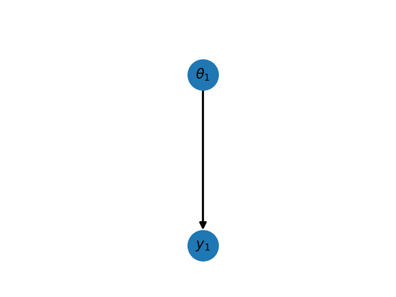
As you can see we have added a new CPD $\mathbb{P}(Y_1\mid \theta_1)$ reprented by the canonical form $\phi_2(Y_1,\theta_1,K^\prime,h^\prime,g^\prime)$ which by using (1) and (3) we can see has

$$K^\prime=\Phi\Sigma_{\epsilon}^{-1}\Phi^T, \qquad h^\prime=\Phi^T\Sigma_{\epsilon}^{-1}b,$$

We then combine this conditioned CPD factor with its parent factor (associated with the prior distribution of the parameters $\theta_i$ by multiplying these two factors together after eliminating the data variables from the scope of the CPD. The combined factor has parameters

$$K=\Phi_i\Sigma_{\epsilon_i}^{-1}\Phi_i^T+\Sigma_{ii}^{-1}, \qquad h=\Sigma_{ii}^{-1}\mu_i+\Phi_i^T\Sigma_{\epsilon_i}^{-1}y$$

which represents a Gaussian with mean and covariance given by

$$\Sigma^\mathrm{post}=\left(\Phi_i\Sigma_{\epsilon_i}^{-1}\Phi_i^T+\Sigma_{ii}^{-1}\right)^{-1}, \qquad \mu^\mathrm{post} = \Sigma^\mathrm{post}\left(\Sigma_{ii}^{-1}\mu_i+\Phi_i^T\Sigma_{\epsilon_i}^{-1}y\right)$$

which is just the usual expression for the posterior of a gaussian linear model using only the linear model, noise and prior associated with a single node. Here we used the relationship between the canonical factors and the covariance $C$ and mean $m$ of the equivalent Gaussian distribution

$$C=K^{-1}, \qquad m=Ch$$

Let’s compute the posterior with this procedure

network.convert_to_compact_factors()

noise = [noise_std[ii]*np.random.normal(
    0,noise_std[ii],(nsamples[ii],1))]
values_train=[b.dot(c)+s+n for b,c,s,n in zip(
    data_cpd_mats,true_coefs,data_cpd_vecs,noise)]

evidence, evidence_ids = network.assemble_evidence(values_train)


for factor in network.factors:
    factor.condition(evidence_ids,evidence)
factor_post = network.factors[0]
for jj in range(1, len(network.factors)):
    factor_post *= network.factors[jj]
gauss_post = convert_gaussian_from_canonical_form(
    factor_post.precision_matrix,factor_post.shift)

We can check this matches the posterior returned by the classical formulas

from pyapprox.bayesian_inference.laplace import \
    laplace_posterior_approximation_for_linear_models
true_post = laplace_posterior_approximation_for_linear_models(
    data_cpd_mats[0],prior_means[ii]*np.ones((nparams[0],1)),
    np.linalg.inv(prior_covs[ii]*np.eye(nparams[0])),
    np.linalg.inv(noise_covs[0]),values_train[0],data_cpd_vecs[0])

assert np.allclose(gauss_post[1],true_post[1])
assert np.allclose(gauss_post[0],true_post[0].squeeze())

Marginalizing Canonical Forms

Gaussian networks are best used when one wants to comute a marginal of the joint density of parameters, possibly conditioned on data. The following describes the process of marginalization and conditioning often referred to as the sum-product eliminate variable algorithm.

First lets discuss how to marginalize a canoncial form, e.g. compute

$$\int \phi(X,Y,K,h,g)dY$$

which marginalizes out the variable $Y$ from a canonical form also involving the variable $X$. Provided $K_{YY}$ in (2) is positive definite the marginalized canonical form has parameters

$$K^\prime=K_{XX}-K_{XY}K_{YY}^{-1}K_{YX},\quad h^\prime=h_X-K_{XY}K_{YY}^{-1}h_{Y}, \quad g^\prime=g+h_Y^Ty-\frac{1}{2}y^TK_{YY}y$$

Computing the marginal density of a network conditioned on data

Again consider a three model recursive network

nnodes = 3
graph = nx.DiGraph()
prior_covs = [1,2,3]
prior_means = [-1,-2,-3]
cpd_scales  =[0.5,0.4]
node_labels = [f'Node_{ii}' for ii in range(nnodes)]
nparams = np.array([2]*3)
cpd_mats  = [None,cpd_scales[0]*np.eye(nparams[1],nparams[0]),
             cpd_scales[1]*np.eye(nparams[2],nparams[1])]

ii=0
graph.add_node(
    ii,label=node_labels[ii],cpd_cov=prior_covs[ii]*np.eye(nparams[ii]),
    nparams=nparams[ii],cpd_mat=cpd_mats[ii],
    cpd_mean=prior_means[ii]*np.ones((nparams[ii],1)))
for ii in range(1,nnodes):
    cpd_mean = np.ones((nparams[ii],1))*(
        prior_means[ii]-cpd_scales[ii-1]*prior_means[ii-1])
    cpd_cov = np.eye(nparams[ii])*max(
        1e-8,prior_covs[ii]-cpd_scales[ii-1]**2*prior_covs[ii-1])
    graph.add_node(ii,label=node_labels[ii],cpd_cov=cpd_cov,
                   nparams=nparams[ii],cpd_mat=cpd_mats[ii],
                   cpd_mean=cpd_mean)

graph.add_edges_from([(ii,ii+1) for ii in range(nnodes-1)])

nsamples = [3]*nnodes
noise_std=[0.01]*nnodes
data_cpd_mats=[np.random.normal(0,1,(nsamples[ii],nparams[ii]))
               for ii in range(nnodes)]
data_cpd_vecs=[np.ones((nsamples[ii],1)) for ii in range(nnodes)]
true_coefs=[np.random.normal(0,np.sqrt(prior_covs[ii]),(nparams[ii],1))
            for ii in range(nnodes)]
noise_covs=[np.eye(nsamples[ii])*noise_std[ii]**2
            for ii in range(nnodes)]

network = GaussianNetwork(graph)
network.add_data_to_network(data_cpd_mats,data_cpd_vecs,noise_covs)

noise = [noise_std[ii]*np.random.normal(
    0,noise_std[ii],(nsamples[ii],1)) for ii in range(nnodes)]
values_train=[b.dot(c)+s+n for b,c,s,n in zip(
    data_cpd_mats,true_coefs,data_cpd_vecs,noise)]

evidence, evidence_ids = network.assemble_evidence(values_train)

fig,ax=plt.subplots(1,1,figsize=(8,6))
plot_hierarchical_network_network_with_data(network.graph,ax)
#plt.show()

The sum-product eliminate variable algorithm begins by first conditioning all the network factors on the available data and then finding the ids of the variables o eliminate from the factors. Let the scope of the entire network be $\Psi$, e.g. for this example $\Phi=\{\theta_1,\theta_2,\theta_3,Y_1,Y_2,Y_3\}$ if we wish to compute the $\theta_3$ marginal, i.e. marginalize out all other variables, the variables that need to be eliminated will be associated with the nodes $\Phi\setminus\; \left(\{\theta_3\}\cap\{Y_1,Y_2,Y_3\}\right) =\{\theta_1,\theta_2\}$. Variables associated with evidence (data) should not be identified for elimination (marginalization).

network.convert_to_compact_factors()
for factor in network.factors:
     factor.condition(evidence_ids,evidence)

query_labels = [node_labels[2]]
eliminate_ids = get_var_ids_to_eliminate_from_node_query(
    network.node_var_ids,network.node_labels,query_labels,evidence_ids)

Once the variables to eliminate have been identified, they are marginalized out of any factor in which they are present; other factors are left untouched. The marginalized factors are then multiplied with the remaining factors to compute the desired marginal density using the sum product variable elimination algorithm.

factor_post = sum_product_variable_elimination(network.factors,eliminate_ids)

gauss_post = convert_gaussian_from_canonical_form(
    factor_post.precision_matrix,factor_post.shift)

print('Posterior Mean\n',gauss_post[0])
print('Posterior Covariance\n',gauss_post[1])

Out:

Posterior Mean
 [-0.36647195  1.0164208 ]
Posterior Covariance
 [[ 6.33358021e-03 -5.39518433e-04]
 [-5.39518433e-04  6.51970946e-05]]

References

KFPGM2009

Probabilistic Graphical Models: Principles and Techinques. 2009