Note
Click here to download the full example code
Sensitivity Analysis
Quantifying the sensitivity of a model output \(f\) to the model parameters \(\rv\) can be an important component of any modeling exercise. This section demonstrates how to use opoular local and global sensitivity analysis.
Sobol Indices
Any function \(f\) with finite variance parameterized by a set of independent variables \(\rv\) with \(\pdf(\rv)=\prod_{j=1}^d\pdf(\rv_j)\) and support \(\rvdom=\bigotimes_{j=1}^d\rvdom_j\) can be decomposed into a finite sum, referred to as the ANOVA decomposition,
or more compactly
where \(\hat{f}_\V{u}\) quantifies the dependence of the function \(f\) on the variable dimensions \(i\in\V{u}\) and \(\V{u}=(u_1,\ldots,u_s)\subseteq\mathcal{D}=\{1,\ldots,d\}\).
The functions \(\hat{f}_\V{u}\) can be obtained by integration, specifically
where \(\dx{\pdf_{\mathcal{D} \setminus \V{u}}(\rv)}=\prod_{j\notin\V{u}}\dx{\pdf_j(\rv)}\) and \(\rvdom_{\mathcal{D} \setminus \V{u}}=\bigotimes_{j\notin\V{u}}\rvdom_j\).
The first-order terms \(\hat{f}_{\V{u}}(\rv_i)\), \(\lVert \V{u}\rVert_{0}=1\) represent the effect of a single variable acting independently of all others. Similarly, the second-order terms \(\lVert\V{u}\rVert_{0}=2\) represent the contributions of two variables acting together, and so on.
The terms of the ANOVA expansion are orthogonal, i.e. the weighted \(L^2\) inner product \((\hat{f}_\V{u},\hat{f}_\V{v})_{L^2_\pdf}=0\), for \(\V{u}\neq\V{v}\). This orthogonality facilitates the following decomposition of the variance of the function \(f\)
where \(\dx{\pdf_{\V{u}}(\rv)}=\prod_{j\in\V{u}}\dx{\pdf_j(\rv)}\).
The quantities \(\var{\hat{f}_\V{u}}/ \var{f}\) are referred to as Sobol indices [SMCS2001] and are frequently used to estimate the sensitivity of \(f\) to single, or combinations of input parameters. Note that this is a global sensitivity, reflecting a variance attribution over the range of the input parameters, as opposed to the local sensitivity reflected by a derivative. Two popular measures of sensitivity are the main effect and total effect indices given respectively by
where \(\V{e}_i\) is the unit vector, with only one non-zero entry located at the \(i\)-th element, and \(\mathcal{J} = \{\V{u}:i\in\V{u}\}\).
Sobol indices can be computed different ways. In the following we will use polynomial chaos expansions, as in [SRESS2008].
import numpy as np
import pyapprox as pya
from pyapprox.benchmarks.benchmarks import setup_benchmark
from pyapprox.approximate import approximate
benchmark = setup_benchmark("ishigami",a=7,b=0.1)

num_samples = 1000
train_samples=pya.generate_independent_random_samples(
    benchmark.variable,num_samples)
train_vals = benchmark.fun(train_samples)

approx_res = approximate(
    train_samples,train_vals,'polynomial_chaos',
    {'basis_type':'hyperbolic_cross','variable':benchmark.variable,
     'options':{'max_degree':8}})
pce = approx_res.approx

res = pya.analyze_sensitivity_polynomial_chaos(pce)
Now lets compare the estimated values with the exact value
print(res.main_effects[:,0])
print(benchmark.main_effects[:,0])
Out:
[3.14720223e-01 4.41237311e-01 7.54746362e-07]
[0.31390519 0.44241114 0.        ]
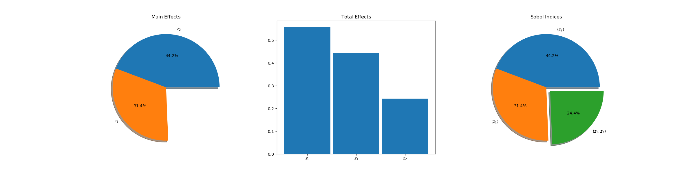
We can visualize the sensitivity indices using the following
import matplotlib.pyplot as plt
fig,axs = plt.subplots(1,3,figsize=(3*8,6))
pya.plot_main_effects(benchmark.main_effects,axs[0])
pya.plot_total_effects(benchmark.total_effects,axs[1])
pya.plot_interaction_values(benchmark.sobol_indices,benchmark.sobol_interaction_indices,axs[2])
axs[0].set_title(r'$\mathrm{Main\;Effects}$')
axs[1].set_title(r'$\mathrm{Total\;Effects}$')
axs[2].set_title(r'$\mathrm{Sobol\;Indices}$')
plt.show()