Note
Go to the end to download the full example code
Univariate Interpolation
This tutorial will present methods to approximate univariate functions \(\hat{f}_{\alpha}:\reals\to\reals\) using interpolation. An interpolant of a function \(f\) is a weighted linear combination of basis functions
where the weights are the evaluation on the function \(f\) on a set of points \(\rv_i^{(j)}, j=1\ldots,M_\beta\). Here \(\beta\) is an index that controls the number of points in the interpolant and the indices \(\alpha\) and \(i\) can be ingored in this tutorial.
I included \(\alpha\) and \(i\) because they will be useful in later tutotorials that build multi-fidelity multi-variate interpolants of functions \(f_\alpha:\reals^D\to\reals\). In such cases i is used to denote the dimension \(i=1\ldots,D\) and \(\alpha\) is an index functions of different accuracy (fidelity).
The properties of interpolants depends on two factors. The way the interpolation points \(\rv_i^{(j)}\) are constructed and the form of the basis functions \(\phi\).
In this tutorial I will introduce two types on interpolation strategies based on local and global basis functions.
Lagrange Interpolation
Lagrange interpolation uses global polynomials as basis functions
The error of a Lagrange interpolant on the interval \([a,b]\) is given by
where \(f_\alpha^{(n+1)}(c)\) is the (n+1)-th derivative of the function at some point in \(c\in[a,b]\).
The error in the polynomial is bounded by
This result shows that the choice of inteprolation points matter. Specificallly, we can not change the derivatives of a function but we can attempt to minimize
Chebyshev points are a very good choice of interpolation points that produce a small value of the quantity above. They are given by
Piecewise polynomial interpolation
A proof of this lemma can be found here
import numpy as np
import matplotlib.pyplot as plt

from pyapprox.surrogates.interp.tensorprod import (
    UnivariatePiecewiseQuadraticBasis, UnivariateLagrangeBasis,
    TensorProductInterpolant)


#The following code compares polynomial and piecewise polynomial univariate basis functions.
nnodes = 5
samples = np.linspace(-1, 1, 201)
ax = plt.subplots(1, 2, figsize=(2*8, 6), sharey=True)[1]
cheby_nodes = np.cos(np.arange(nnodes)*np.pi/(nnodes-1))
lagrange_basis = UnivariateLagrangeBasis()
lagrange_basis_vals = lagrange_basis(cheby_nodes, samples)
ax[0].plot(samples, lagrange_basis_vals)
ax[0].plot(cheby_nodes, cheby_nodes*0, 'ko')
equidistant_nodes = np.linspace(-1, 1, nnodes)
quadratic_basis = UnivariatePiecewiseQuadraticBasis()
piecewise_basis_vals = quadratic_basis(equidistant_nodes, samples)
_ = ax[1].plot(samples, piecewise_basis_vals)
_ = ax[1].plot(equidistant_nodes, equidistant_nodes*0, 'ko')
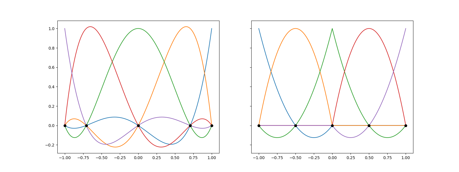
Notice that the unlike the lagrange basis the picewise polynomial basis is non-zero only on a local region of the input space.
The compares the accuracy of lagrange basis the picewise polynomial approximations for a piecewise continuous function
def fun(samples):
    yy = samples[0].copy()
    yy[yy > 1/3] = 1.0
    yy[yy <= 1/3] = 0.
    return yy[:, None]


lagrange_interpolant = TensorProductInterpolant([lagrange_basis])
quadratic_interpolant = TensorProductInterpolant([quadratic_basis])
axs = plt.subplots(1, 2, figsize=(2*8, 6))[1]
[ax.plot(samples, fun(samples[None, :])) for ax in axs]
cheby_nodes = -np.cos(np.arange(nnodes)*np.pi/(nnodes-1))
values = fun(cheby_nodes[None, :])
lagrange_interpolant.fit([cheby_nodes], values)
equidistant_nodes = np.linspace(-1, 1, nnodes)
values = fun(equidistant_nodes[None, :])
quadratic_interpolant.fit([equidistant_nodes], values)
axs[0].plot(samples, lagrange_interpolant(samples[None, :]), ':')
axs[0].plot(cheby_nodes, values, 'o')
axs[1].plot(samples, quadratic_interpolant(samples[None, :]), '--')
_ = axs[1].plot(equidistant_nodes, values, 's')
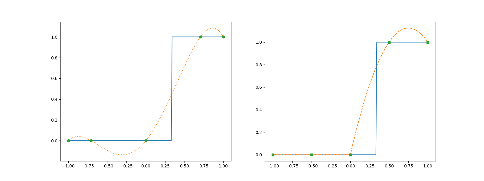
The Lagrange polynomials induce oscillations around the discontinuity, which significantly decreases the convergence rate of the approximation. The picewise quadratic also over and undershoots around the discontinuity, but the phenomena is localized.
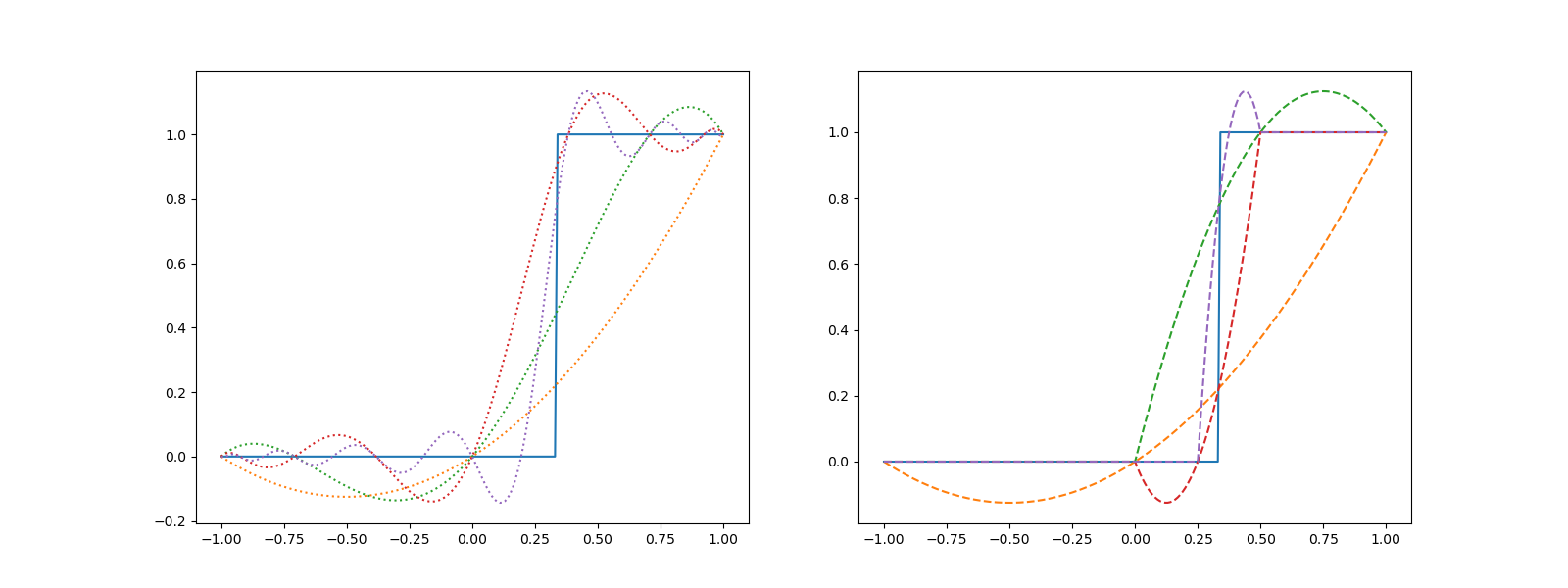
Now lets see how the error changes as we increase the number of nodes
axs = plt.subplots(1, 2, figsize=(2*8, 6))[1]
[ax.plot(samples, fun(samples[None, :])) for ax in axs]
for nnodes in [3, 5, 9, 17]:
    nodes = np.cos(np.arange(nnodes)*np.pi/(nnodes-1))
    values = fun(nodes[None, :])
    lagrange_interpolant.fit([nodes], values)
    nodes = np.linspace(-1, 1, nnodes)
    values = fun(nodes[None, :])
    quadratic_interpolant.fit([nodes], values)
    axs[0].plot(samples, lagrange_interpolant(samples[None, :]), ':')
    _ = axs[1].plot(samples, quadratic_interpolant(samples[None, :]), '--')
Probability aware interpolation for UQ
When interpolants are used for UQ we do not need the approximation to be accurate everywhere but rather only in regions of high-probability. First lets see what happens when we approximate a function using an interpolant that targets accuracy with respect to a dominating measure \(\nu\) when really needed an approximation that targets accuracy with respect to a different measure \(w\).
from scipy import stats
from pyapprox.variables.joint import IndependentMarginalsVariable
from pyapprox.benchmarks import setup_benchmark
from pyapprox.surrogates.orthopoly.quadrature import (
    gauss_jacobi_pts_wts_1D)
from pyapprox.util.utilities import cartesian_product

nvars = 1
c = np.array([20])
w = np.array([0])
benchmark = setup_benchmark(
    "genz", test_name="oscillatory", nvars=nvars, coeff=[c, w])

alpha_stat, beta_stat = 11, 11
true_rv = IndependentMarginalsVariable(
    [stats.beta(a=alpha_stat, b=beta_stat)]*nvars)

interp = TensorProductInterpolant([lagrange_basis]*nvars)
opt_interp = TensorProductInterpolant([lagrange_basis]*nvars)

alpha_poly, beta_poly = 0, 0
ntrain_samples = 7
xx = gauss_jacobi_pts_wts_1D(ntrain_samples, alpha_poly, beta_poly)[0]
train_samples = cartesian_product([(xx+1)/2]*nvars)
train_values = benchmark.fun(train_samples)
interp.fit(train_samples, train_values)

opt_xx = gauss_jacobi_pts_wts_1D(ntrain_samples, beta_stat-1, alpha_stat-1)[0]
opt_train_samples = cartesian_product([(opt_xx+1)/2]*nvars)
opt_train_values = benchmark.fun(opt_train_samples)
opt_interp.fit(opt_train_samples, opt_train_values)


ax = plt.subplots(1, 1, figsize=(8, 6))[1]
plot_xx = np.linspace(0, 1, 101)
true_vals = benchmark.fun(plot_xx[None, :])
pbwt = r"\pi"
ax.plot(plot_xx, true_vals, '-r', label=r'$f(z)$')
ax.plot(plot_xx, interp(plot_xx[None, :]), ':k', label=r'$f_M^\nu$')
ax.plot(train_samples[0], train_values[:, 0], 'ko', ms=10,
        label=r'$\mathcal{Z}_{M}^{\nu}$')
ax.plot(plot_xx, opt_interp(plot_xx[None, :]), '--b', label=r'$f_M^%s$' % pbwt)
ax.plot(opt_train_samples[0], opt_train_values[:, 0], 'bs',
        ms=10, label=r'$\mathcal{Z}_M^%s$' % pbwt)

pdf_vals = true_rv.pdf(plot_xx[None, :])[:, 0]
ax.set_ylim(true_vals.min()-0.1*abs(true_vals.min()),
            max(true_vals.max(), pdf_vals.max())*1.1)
ax.fill_between(
    plot_xx, ax.get_ylim()[0], pdf_vals+ax.get_ylim()[0],
    alpha=0.3, visible=True,
    label=r'$%s(z)$' % pbwt)
ax.set_xlabel(r'$M$', fontsize=24)
_ = ax.legend(fontsize=18, loc="upper right")
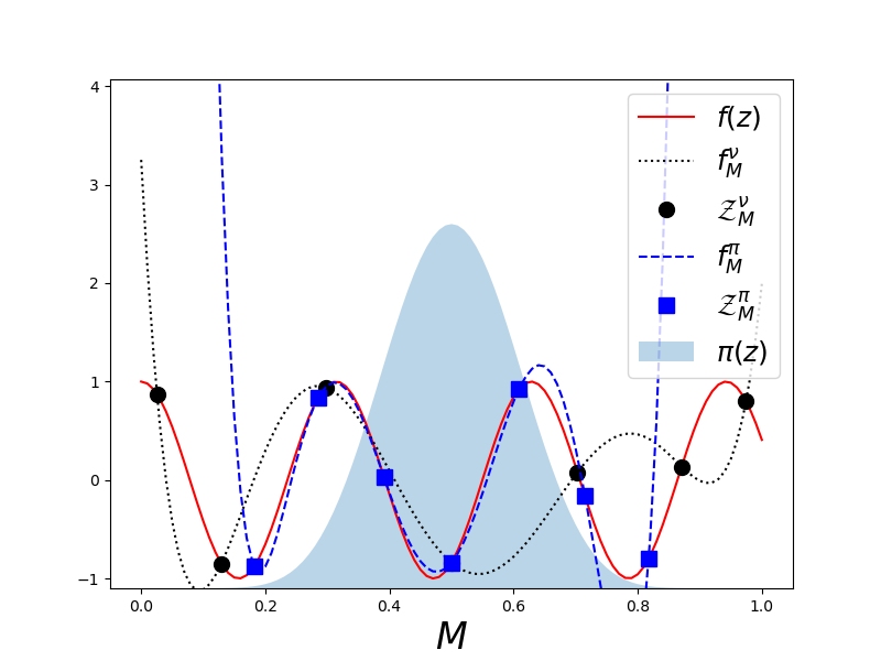
As you can see the approximation that targets the uniform norm is “more accurate” on average over the domain, but the interpolant that directly targets accuracy with respect to the desired Beta distribution is more accurate in the regions of non-negligible probability.
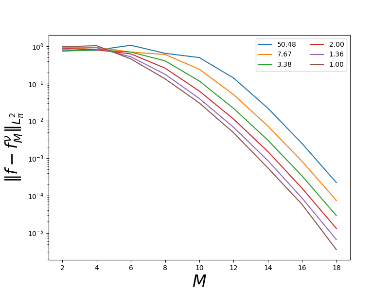
Now lets looks at how the accuracy changes with the “distance” between the dominating and target measures. This demonstrates the numerical impact of the main theorem in [XJD2013].
def compute_density_ratio_beta(num, true_rv, alpha_stat_2, beta_stat_2):
    beta_rv2 = IndependentMarginalsVariable(
        [stats.beta(a=alpha_stat_2, b=beta_stat_2)]*nvars)
    print(beta_rv2, true_rv)
    xx = np.random.uniform(0, 1, (nvars, 100000))
    density_ratio = true_rv.pdf(xx)/beta_rv2.pdf(xx)
    II = np.where(np.isnan(density_ratio))[0]
    assert II.shape[0] == 0
    return density_ratio.max()


def compute_L2_error(interp, validation_samples, validation_values):
    nvalidation_samples = validation_values.shape[0]
    approx_vals = interp(validation_samples)
    l2_error = np.linalg.norm(validation_values-approx_vals)/np.sqrt(
        nvalidation_samples)
    return l2_error


nvars = 3
c = np.array([20, 20, 20])
w = np.array([0, 0, 0])
benchmark = setup_benchmark(
    "genz", test_name="oscillatory", nvars=nvars, coeff=[c, w])
true_rv = IndependentMarginalsVariable(
    [stats.beta(a=alpha_stat, b=beta_stat)]*nvars)

nvalidation_samples = 1000
validation_samples = true_rv.rvs(nvalidation_samples)
validation_values = benchmark.fun(validation_samples)
interp = TensorProductInterpolant([lagrange_basis]*nvars)

alpha_polys = np.arange(0., 11., 2.)
ntrain_samples_list = np.arange(2, 20, 2)
ax = plt.subplots(1, 1, figsize=(8, 6))[1]
for alpha_poly in alpha_polys:
    beta_poly = alpha_poly
    density_ratio = compute_density_ratio_beta(
        nvars, true_rv, beta_poly+1, alpha_poly+1)
    results = []
    for ntrain_samples in ntrain_samples_list:
        xx = gauss_jacobi_pts_wts_1D(ntrain_samples, alpha_poly, beta_poly)[0]
        nodes_1d = [(xx+1)/2]*nvars
        train_samples = cartesian_product(nodes_1d)
        train_values = benchmark.fun(train_samples)
        interp.fit(nodes_1d, train_values)
        l2_error = compute_L2_error(
            interp, validation_samples, validation_values)
        results.append(l2_error)
    ax.semilogy(ntrain_samples_list, results,
                label="{0:1.2f}".format(density_ratio))

ax.set_xlabel(r'$M$', fontsize=24)
ax.set_ylabel(r'$\| f-f_M^\nu\|_{L^2_%s}$' % pbwt, fontsize=24)
_ = ax.legend(ncol=2)
Independent Marginal Variable
Number of variables: 3
Unique variables and global id:
    beta(a=1.0,b=1.0,loc=[0],scale=[1]): z0, z1, z2 Independent Marginal Variable
Number of variables: 3
Unique variables and global id:
    beta(a=11,b=11,loc=[0],scale=[1]): z0, z1, z2
Independent Marginal Variable
Number of variables: 3
Unique variables and global id:
    beta(a=3.0,b=3.0,loc=[0],scale=[1]): z0, z1, z2 Independent Marginal Variable
Number of variables: 3
Unique variables and global id:
    beta(a=11,b=11,loc=[0],scale=[1]): z0, z1, z2
Independent Marginal Variable
Number of variables: 3
Unique variables and global id:
    beta(a=5.0,b=5.0,loc=[0],scale=[1]): z0, z1, z2 Independent Marginal Variable
Number of variables: 3
Unique variables and global id:
    beta(a=11,b=11,loc=[0],scale=[1]): z0, z1, z2
Independent Marginal Variable
Number of variables: 3
Unique variables and global id:
    beta(a=7.0,b=7.0,loc=[0],scale=[1]): z0, z1, z2 Independent Marginal Variable
Number of variables: 3
Unique variables and global id:
    beta(a=11,b=11,loc=[0],scale=[1]): z0, z1, z2
Independent Marginal Variable
Number of variables: 3
Unique variables and global id:
    beta(a=9.0,b=9.0,loc=[0],scale=[1]): z0, z1, z2 Independent Marginal Variable
Number of variables: 3
Unique variables and global id:
    beta(a=11,b=11,loc=[0],scale=[1]): z0, z1, z2
Independent Marginal Variable
Number of variables: 3
Unique variables and global id:
    beta(a=11.0,b=11.0,loc=[0],scale=[1]): z0, z1, z2 Independent Marginal Variable
Number of variables: 3
Unique variables and global id:
    beta(a=11,b=11,loc=[0],scale=[1]): z0, z1, z2
References
Total running time of the script: ( 0 minutes 1.675 seconds)