Note
Go to the end to download the full example code
Push Forward Based Inference
This tutorial describes push forward based inference (PFI) [BJWSISC2018].
PFI solves the inverse problem of inferring parameters \(\rv\) of a deterministic model \(f(\rv)\) from stochastic observational data on quantities of interest. The solution is a posterior probability measure that when propagated through the deterministic model produces a push-forward measure that exactly matches a given observed probability measure on available data.
The solution to the PFI inverse problem is given by
where \(\pi_\text{pr}(\rv)\) is a prior density which captures any initial knowledge, \(\pi_\text{obs}(f(\rv))\) is the density on the observations, and \(\pi_\text{model}(f(\rv))\) is the push-forward of the prior density trough the forward model.
import numpy as np
import matplotlib.pyplot as plt
import matplotlib as mpl
from scipy import stats
First we must define the forward model. We will use a functional of solution to the following system of non-linear equations
Specifically we choose \(f(\rv)=x_2(\rv)\).
from pyapprox.benchmarks import setup_benchmark
benchmark = setup_benchmark("parameterized_nonlinear_model")
model = benchmark.fun
Define the prior density and the observational density
prior_variable = benchmark.variable
prior_pdf = prior_variable.pdf


mean = 0.3
variance = 0.025**2
obs_variable = stats.norm(mean, np.sqrt(variance))
def obs_pdf(y): return obs_variable.pdf(y)
PFI requires the push forward of the prior \(\pi_\text{model}(f(\rv))\). Lets approximate this PDF using a Gaussian kernel density estimate built on a large number model outputs evaluated at random samples of the prior.
#Define samples used to evaluate the push forward of the prior
num_prior_samples = 10000
prior_samples = prior_variable.rvs(num_prior_samples)
response_vals_at_prior_samples = model(prior_samples)

#Construct a KDE of the push forward of the prior through the model
push_forward_kde = stats.gaussian_kde(response_vals_at_prior_samples.T)
def push_forward_pdf(y): return push_forward_kde(y.T)[:, None]
We can now simply evaluate
using the approximate push forward PDF \(\hat{\pi}_\text{model}(f(\rv))\). Lets use this fact to plot the posterior density.
#Define the samples at which to evaluate the posterior density
num_pts_1d = 50
from pyapprox.analysis import visualize
X, Y, samples_for_posterior_eval = \
    visualize.get_meshgrid_samples_from_variable(prior_variable, 30)

#Evaluate the density of the prior at the samples used to evaluate
#the posterior
prior_prob_at_samples_for_posterior_eval = prior_pdf(
    samples_for_posterior_eval)

#Evaluate the model at the samples used to evaluate
#the posterior
response_vals_at_samples_for_posterior_eval = model(samples_for_posterior_eval)

#Evaluate the distribution on the observable data
obs_prob_at_samples_for_posterior_eval = obs_pdf(
    response_vals_at_samples_for_posterior_eval)

#Evaluate the probability of the responses at the desired points
response_prob_at_samples_for_posterior_eval = push_forward_pdf(
    response_vals_at_samples_for_posterior_eval)

#Evaluate the posterior probability
posterior_prob = (prior_prob_at_samples_for_posterior_eval*(
    obs_prob_at_samples_for_posterior_eval /
    response_prob_at_samples_for_posterior_eval))

#Plot the posterior density
p = plt.contourf(
    X, Y, np.reshape(posterior_prob, X.shape),
    levels=np.linspace(posterior_prob.min(), posterior_prob.max(), 30),
    cmap=mpl.cm.coolwarm)
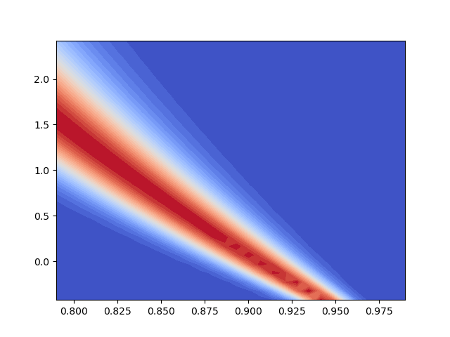
Note that to plot the posterior we had to evaluate the model at each plot points. This can be expensive. To avoid this surrogate models can be used to replace the expensive model [BJWSISC2018b]. But ignoring such approaches we can still obtain useful information without additional model evaluations as is done above. For example, we can easily and with no additional model evaluations evaluate the posterior density at the prior samples
prior_prob_at_prior_samples = prior_pdf(prior_samples)
obs_prob_at_prior_samples = obs_pdf(response_vals_at_prior_samples)
response_prob_at_prior_samples = push_forward_pdf(
    response_vals_at_prior_samples)
posterior_prob_at_prior_samples = prior_prob_at_prior_samples * (
    obs_prob_at_prior_samples / response_prob_at_prior_samples)
We can also use rejection sampling to draw samples from the posterior Given a random number \(u\sim U[0,1]\), and the prior samples \(x\). We accept a prior sample as a draw from the posterior if
for some proposal density \(\pi_\text{prop}(\rv)\) such that \(M\pi_\text{prop}(\rv)\) is an upper bound on the density of the posterior. Here we set \(M=1.1\,\max_{\rv\in\rvdom}\pi_\text{post}(\rv)\) to be a constant sligthly bigger than the maximum of the posterior over all the prior samples.
max_posterior_prob = posterior_prob_at_prior_samples.max()
accepted_samples_idx = np.where(
    posterior_prob_at_prior_samples/(1.1*max_posterior_prob) >
    np.random.uniform(0., 1., (num_prior_samples, 1)))[0]
posterior_samples = prior_samples[:, accepted_samples_idx]
acceptance_ratio = posterior_samples.shape[1]/num_prior_samples
print("Acceptance ratio", acceptance_ratio)

#plot the accepted samples
plt.plot(posterior_samples[0, :], posterior_samples[1, :], 'ok')
plt.xlim(model.ranges[:2])
_ = plt.ylim(model.ranges[2:])
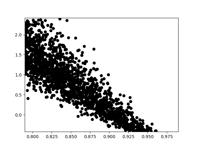
Acceptance ratio 0.172
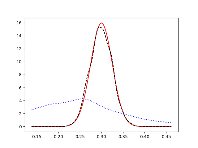
The goal of inverse problem was to define the posterior density that when push forward through the forward model exactly matches the observed PDF. Lets check that by pushing forward our samples from the posterior.
#compute the posterior push forward
posterior_push_forward_kde = stats.gaussian_kde(
    response_vals_at_prior_samples[accepted_samples_idx].T)


def posterior_push_forward_pdf(
    y): return posterior_push_forward_kde(y.T).squeeze()


plt.figure()
lb, ub = obs_variable.interval(1-1e-10)
y = np.linspace(lb, ub, 101)
plt.plot(y, obs_pdf(y), 'r-')
plt.plot(y, posterior_push_forward_pdf(y), 'k--')
plt.plot(y, push_forward_pdf(y), 'b:')
plt.show()
Explore the number effect of changing the number of prior samples on the posterior and its push-forward.
References
Total running time of the script: ( 0 minutes 0.672 seconds)