A simple PDE problem

In this first example, we will construct a finite element discretization of a classical PDE problem and solve it. The full code of this example can be found in examples/example_pde.py in the PyNucleus repository.

Factories

The creation of different groups of objects, such as finite element spaces or meshes, use factories. The available classes that a factory provides can be displayed by calling the print() function on it. An object is built by passing the name of the desired class and additional parameters to the factory. If this sounds vague now, don’t worry, the examples below will make it clear.

Meshes

The first object we need to create is a mesh to support the finite element discretization. The output of the code snippet is given below.

import matplotlib.pyplot as plt
from PyNucleus import meshFactory
print(meshFactory)

Available:
'simpleInterval' with aliases ['interval'], signature: '(a=0.0, b=1.0, numCells=1)'
'unitInterval', signature: '(a=0.0, b=1.0, numCells=1)'
'intervalWithInteraction', signature: '(a, b, horizon, h=None, strictInteraction=True)'
'disconnectedInterval', signature: '(sep=0.1)'
'simpleSquare', signature: '()'
'crossSquare' with aliases ['squareCross'], signature: '()'
'unitSquare' with aliases ['square', 'rectangle'], signature: '(N=2, M=None, ax=0, ay=0, bx=1, by=1, crossed=False, preserveLinesHorizontal=[], preserveLinesVertical=[], xVals=None, yVals=None)'
'gradedSquare', signature: '(factor=0.6)'
'gradedBox' with aliases ['gradedCube'], signature: '(factor=0.6)'
'squareWithInteraction', signature: '(ax, ay, bx, by, horizon, h=None, uniform=False, strictInteraction=True, innerRadius=-1, preserveLinesHorizontal=[], preserveLinesVertical=[], **kwargs)'
'simpleLshape' with aliases ['Lshape', 'L-shape'], signature: '()'
'circle' with aliases ['disc', 'unitDisc', 'ball2d', '2dball'], signature: '(n, radius=1.0, returnFacets=False, projectNodeToOrigin=True, **kwargs)'
'graded_circle' with aliases ['gradedCircle'], signature: '(M, mu=2.0, radius=1.0, returnFacets=False, **kwargs)'
'discWithInteraction', signature: '(radius, horizon, h=0.25, max_volume=None, projectNodeToOrigin=True)'
'twinDisc', signature: '(n, radius=1.0, sep=0.1, **kwargs)'
'dumbbell', signature: '(n=8, radius=1.0, barAngle=0.7853981633974483, barLength=3, returnFacets=False, minAngle=30, **kwargs)'
'wrench', signature: '(n=8, radius=0.17, radius2=0.3, barLength=2, returnFacets=False, minAngle=30, **kwargs)'
'cutoutCircle' with aliases ['cutoutDisc'], signature: '(n, radius=1.0, cutoutAngle=1.5707963267948966, returnFacets=False, minAngle=30, **kwargs)'
'squareWithCircularCutout', signature: '(ax=-3.0, ay=-3.0, bx=3.0, by=3.0, radius=1.0, num_points_per_unit_len=2)'
'boxWithBallCutout' with aliases ['boxMinusBall'], signature: '(ax=-3.0, ay=-3.0, az=-3.0, bx=3.0, by=3.0, bz=3.0, radius=1.0, points=4, radial_subdiv=None, **kwargs)'
'simpleBox' with aliases ['unitBox', 'cube', 'unitCube'], signature: '()'
'box', signature: '(ax=0.0, ay=0.0, az=0.0, bx=1.0, by=1.0, bz=1.0, Nx=2, Ny=2, Nz=2)'
'ball', signature: '
    Build mesh for 3D ball as surface of revolution.
    points         determines the number of points on the curve.
    radial_subdiv  determines the number of steps in the rotation.
    '
'simpleFicheraCube' with aliases ['fichera', 'ficheraCube'], signature: '()'
'standardSimplex2D', signature: '()'
'standardSimplex3D', signature: '()'

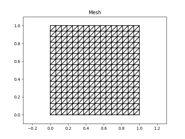
We see what the different meshes that the meshFactory can construct and the default values for associated parameters. We choose to construct a mesh for a square domain \(\Omega=[0, 1] \times [0, 1]\) and refining it uniformly three times:

mesh = meshFactory('square', ax=0., ay=0., bx=1., by=1.)
for _ in range(3):
    mesh = mesh.refine()
print('Mesh:', mesh)

Mesh: mesh2d with 289 vertices and 512 cells

We have created a 2d mesh with 289 vertices and 512 cells. The mesh (as well as many other objects) can be plotted:

plt.figure().gca().set_title('Mesh')
mesh.plot()

Many PyNucleus objects have a plot method, similar to the mesh that we just created.

DoFMaps

In the next step, we create a finite element space on the mesh. By default, we assume a Dirichlet condition on the entire boundary of the domain. We build a piecewise linear finite element space.

from PyNucleus import dofmapFactory
print(dofmapFactory)

Available:
'P0d' with aliases ['P0'], signature: 'P0_DoFMap(meshBase mesh, tag=None, INDEX_t skipCellsAfter=-1)'
'P1c' with aliases ['P1'], signature: 'P1_DoFMap(meshBase mesh, tag=None, INDEX_t skipCellsAfter=-1)'
'P2c' with aliases ['P2'], signature: 'P2_DoFMap(meshBase mesh, tag=None, INDEX_t skipCellsAfter=-1)'
'P3c' with aliases ['P3'], signature: 'P3_DoFMap(meshBase mesh, tag=None, INDEX_t skipCellsAfter=-1)'
'vectorP0d' with aliases ['vectorP0', 'vector-P0', 'vector P0'], signature: '(mesh, *args, **kwargs)'
'vectorP1c' with aliases ['vectorP1', 'vector-P1', 'vector P1'], signature: '(mesh, *args, **kwargs)'
'vectorP2c' with aliases ['vectorP2', 'vector-P2', 'vector P2'], signature: '(mesh, *args, **kwargs)'
'vectorP3c' with aliases ['vectorP3', 'vector-P3', 'vector P3'], signature: '(mesh, *args, **kwargs)'
'N1e', signature: 'N1e_DoFMap(meshBase mesh, tag=None, INDEX_t skipCellsAfter=-1)'

We use a piecewise linear continuous finite element space.

dm = dofmapFactory('P1c', mesh)
print('DoFMap:', dm)

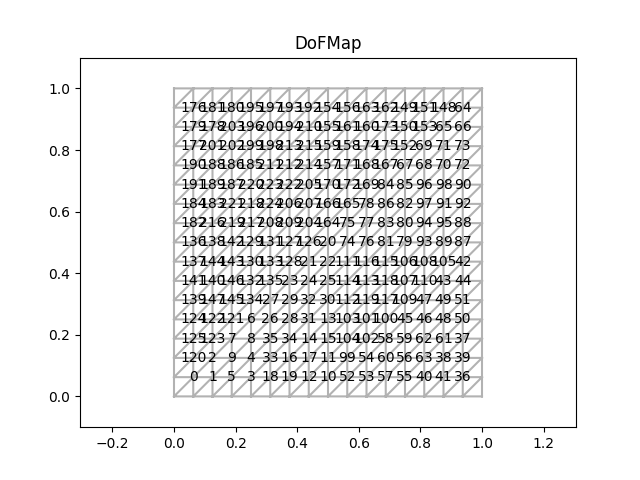
DoFMap: P1 DoFMap with 225 DoFs and 64 boundary DoFs.

By default all degrees of freedom on the boundary of the domain are considered to be “boundary dofs”. The dofmapFactory take an optional second argument that allows to pass an indicator function to control what is considered a boundary dof.

Next, we plot the locations of the degrees of freedom on the mesh.

plt.figure().gca().set_title('DoFMap')
dm.plot()

Functions and vectors

We will be solving the problem

\[\begin{split}-\Delta u &= f & \text{ in } \Omega, \\ u &= 0 & \text{ on } \partial \Omega,\end{split}\]

or, more precisely, its weak form

\[\begin{split}&\text{Find } u \in H^1(\Omega) \text{ such that}\\ &\int_\Omega \nabla u \cdot \nabla v = \int_\Omega fv \qquad\forall v \in H^1_0(\Omega).\end{split}\]

Functions are created using the functionFactory.

from PyNucleus import functionFactory
print(functionFactory)

Available:
'rhsFunSin1D', signature: 'None'
'rhsFunSin2D', signature: '_rhsFunSin2D(INDEX_t k=1, INDEX_t l=1)'
'rhsFunSin3D', signature: 'None'
'solSin1D' with aliases ['sin1d'], signature: '_solSin1D(INDEX_t k=1)'
'solCos1D' with aliases ['cos1d'], signature: '_cos1D(INDEX_t k=1)'
'solSin2D' with aliases ['sin2d'], signature: '_solSin2D(INDEX_t k=1, INDEX_t l=1)'
'solCos2D' with aliases ['cos2d'], signature: 'None'
'solSin3D' with aliases ['sin3d'], signature: '_solSin3D(INDEX_t k=1, INDEX_t l=1, INDEX_t m=1)'
'solFractional', signature: 'solFractional(REAL_t s, INDEX_t dim, REAL_t radius=1.0)'
'solFractionalDerivative', signature: 'solFractionalDerivative(REAL_t s, INDEX_t dim, REAL_t radius=1.0)'
'solFractional1D', signature: 'solFractional1D(REAL_t s, INDEX_t n)'
'solFractional2D', signature: 'solFractional2D(REAL_t s, INDEX_t l, INDEX_t n, REAL_t angular_shift=0.)'
'rhsFractional1D', signature: 'rhsFractional1D(REAL_t s, INDEX_t n)'
'rhsFractional2D', signature: 'rhsFractional2D(REAL_t s, INDEX_t l, INDEX_t n, REAL_t angular_shift=0.)'
'constant', signature: 'constant(REAL_t value)'
'monomial', signature: 'monomial(REAL_t[::1] exponent, REAL_t factor=1.)'
'affine', signature: 'affineFunction(REAL_t[::1] w, REAL_t c)'
'sqrt_affine', signature: 'sqrtAffineFunction(REAL_t[::1] w, REAL_t c)'
'x0', signature: 'monomial(REAL_t[::1] exponent, REAL_t factor=1.)'
'x1', signature: 'monomial(REAL_t[::1] exponent, REAL_t factor=1.)'
'x2', signature: 'monomial(REAL_t[::1] exponent, REAL_t factor=1.)'
'x0**2', signature: 'monomial(REAL_t[::1] exponent, REAL_t factor=1.)'
'x1**2', signature: 'monomial(REAL_t[::1] exponent, REAL_t factor=1.)'
'x2**2', signature: 'monomial(REAL_t[::1] exponent, REAL_t factor=1.)'
'x0*x1', signature: 'monomial(REAL_t[::1] exponent, REAL_t factor=1.)'
'x1*x2', signature: 'monomial(REAL_t[::1] exponent, REAL_t factor=1.)'
'x0*x2', signature: 'monomial(REAL_t[::1] exponent, REAL_t factor=1.)'
'x0**3', signature: 'monomial(REAL_t[::1] exponent, REAL_t factor=1.)'
'x1**3', signature: 'monomial(REAL_t[::1] exponent, REAL_t factor=1.)'
'x2**3', signature: 'monomial(REAL_t[::1] exponent, REAL_t factor=1.)'
'Lambda', signature: 'Lambda(fun)'
'complexLambda', signature: 'complexLambda(fun)'
'squareIndicator', signature: 'squareIndicator(REAL_t[::1] a, REAL_t[::1] b)'
'radialIndicator', signature: 'radialIndicator(REAL_t radius, REAL_t[::1] center=None)'
'rhsBoundaryLayer2D', signature: '_rhsBoundaryLayer2D(REAL_t radius=0.25, REAL_t c=100.0)'
'solBoundaryLayer2D', signature: '_solBoundaryLayer2D(REAL_t radius=0.25, REAL_t c=100.0)'
'solCornerSingularity2D', signature: '_solCornerSingularity2D()'
'solBoundarySingularity2D', signature: 'solBoundarySingularity2D(REAL_t alpha)'
'rhsBoundarySingularity2D', signature: 'rhsBoundarySingularity2D(REAL_t alpha)'
'rhsMotor', signature: 'rhsMotor(coilPairOn=[0, 1, 2])'
'simpleAnisotropy', signature: 'simpleAnisotropy(epsilon=0.1)'
'simpleAnisotropy2', signature: 'simpleAnisotropy2(epsilon=0.1)'
'inclusions', signature: 'inclusions(epsilon=0.1)'
'inclusionsHong', signature: 'inclusionsHong(epsilon=0.1)'
'motorPermeability', signature: 'motorPermeability(epsilon=1.0 / 5200.0, thetaRotor=pi / 12.0, thetaCoil=pi / 32.0, rRotorIn=0.375, rRotorOut=0.5, rStatorIn=0.875, rStatorOut=0.52, rCoilIn=0.8, rCoilOut=0.55, nRotorOut=4, nRotorIn=8, nStatorOut=4, nStatorIn=8)'
'lookup', signature: 'lookupFunction(meshBase mesh, DoFMap dm, REAL_t[::1] u, cellFinder2 cF=None)'
'vectorLookup', signature: 'vectorLookupFunction(meshBase mesh, DoFMap dm, REAL_t[::1] u, cellFinder2 cF=None)'
'shiftScaleFunctor', signature: 'shiftScaleFunctor(function f, REAL_t[::1] shift, REAL_t[::1] scaling)'
'componentVectorFunction' with aliases ['vector'], signature: 'componentVectorFunction(list components)'

We will consider two different forcing functions \(f\). Pointwise evalutated functions such as \(f\) can either be defined in Python, or in Cython. A generic Python function can be used via the Lambda function class.

rhs_1 = functionFactory('Lambda', lambda x: 2*x[0]*(1-x[0]) + 2*x[1]*(1-x[1]))
exact_solution_1 = functionFactory('Lambda', lambda x: x[0]*(1-x[0])*x[1]*(1-x[1]))

The advantage of Cython functions is that their code is compiled, which speeds up evaluation significantly. A couple of compiled functions are already available via the functionFactory.

rhs_2 = functionFactory('rhsFunSin2D')
exact_solution_2 = functionFactory('solSin2D')

We assemble the right-hand side

\[\int_\Omega f v\]

of the linear system by calling the assembleRHS method of the DoFMap object, and interpolate the exact solutions into the finite element space.

b1 = dm.assembleRHS(rhs_1)
u_interp_1 = dm.interpolate(exact_solution_1)

print('Linear system RHS:', b1)
print('Interpolated solution:', u_interp_1)

b2 = dm.assembleRHS(rhs_2)
u_interp_2 = dm.interpolate(exact_solution_2)

Linear system RHS: REALfe_vector<P1 DoFMap with 225 DoFs and 64 boundary DoFs.>
Interpolated solution: REALfe_vector<P1 DoFMap with 225 DoFs and 64 boundary DoFs.>

We plot the interpolated exact solution.

plt.figure().gca().set_title('Interpolated solution')
u_interp_1.plot()

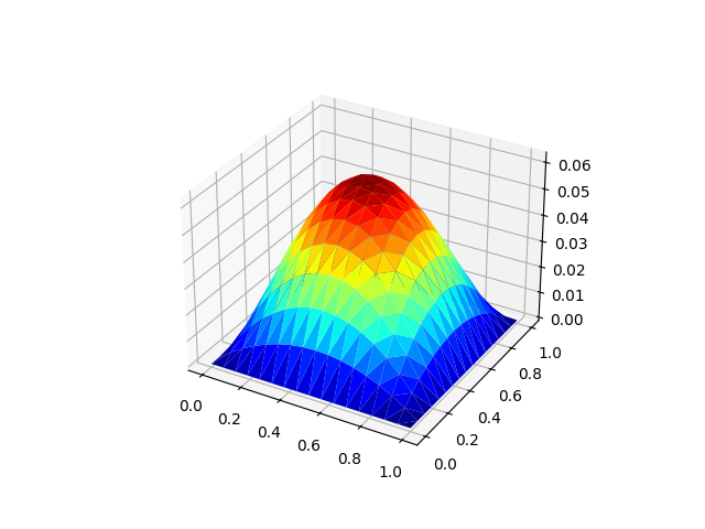
<Axes3D: >

Matrices

We assemble the stiffness matrix associated with the Laplacian

\[\int_\Omega \nabla u \cdot \nabla v\]

laplacian = dm.assembleStiffness()

print('Linear system matrix:', laplacian)

Linear system matrix: <225x225 CSR_LinearOperator with 1457 stored elements>

Solvers

Now that we have assembled our linear system, we want to solve it.

from PyNucleus import solverFactory
print(solverFactory)

Single level solvers:
Available:
'None', signature: 'noop_solver(LinearOperator A, INDEX_t num_rows=-1)'
'lu', signature: 'lu_solver(LinearOperator A, INDEX_t num_rows=-1)'
'chol' with aliases ['cholesky', 'cholmod'], signature: 'chol_solver(LinearOperator A, INDEX_t num_rows=-1)'
'cg', signature: 'cg_solver(LinearOperator A=None, INDEX_t num_rows=-1)'
'gmres', signature: 'gmres_solver(LinearOperator A=None, INDEX_t num_rows=-1)'
'bicgstab', signature: 'bicgstab_solver(LinearOperator A=None, INDEX_t num_rows=-1)'
'ichol', signature: 'ichol_solver(LinearOperator A=None, INDEX_t num_rows=-1)'
'ilu', signature: 'ilu_solver(LinearOperator A=None, INDEX_t num_rows=-1)'
'jacobi' with aliases ['diagonal'], signature: 'jacobi_solver(LinearOperator A=None, INDEX_t num_rows=-1)'
'complex_lu', signature: 'complex_lu_solver(ComplexLinearOperator A, INDEX_t num_rows=-1)'
'complex_gmres', signature: 'complex_gmres_solver(ComplexLinearOperator A=None, INDEX_t num_rows=-1)'
Multi level solvers:
Available:
'mg', signature: 'multigrid(myHierarchyManager, smoother=('jacobi', {'omega': 2.0 / 3.0}), BOOL_t logging=False, **kwargs)'
'complex_mg', signature: 'Complexmultigrid(myHierarchyManager, smoother=('jacobi', {'omega': 2.0 / 3.0}), BOOL_t logging=False, **kwargs)'

We choose to set up an LU direct solver.

solver_direct = solverFactory('lu', A=laplacian)
solver_direct.setup()
print('Direct solver:', solver_direct)

Direct solver: LU

We also set up an iterative solver. Note that we need to specify some additional parameters.

solver_krylov = solverFactory('cg', A=laplacian)
solver_krylov.setup()
solver_krylov.maxIter = 100
solver_krylov.tolerance = 1e-8
print('Krylov solver:', solver_krylov)

Krylov solver: CG(tolerance=1e-08,relTol=0,maxIter=100,2-norm=0)

We allocate a zero vector for the solution of the linear system and solve the equation using the first right-hand side.

u1 = dm.zeros()
solver_direct(b1, u1)

1

We use the interative solver for the second right-hand side.

u2 = dm.zeros()
numIter = solver_krylov(b2, u2)

print('Number of iterations:', numIter)

Number of iterations: 20

We plot the difference between one of the numerical solutions we just computed and the interpolant of the known analytic solution.

plt.figure().gca().set_title('Error')
(u_interp_1-u1).plot(flat=True)

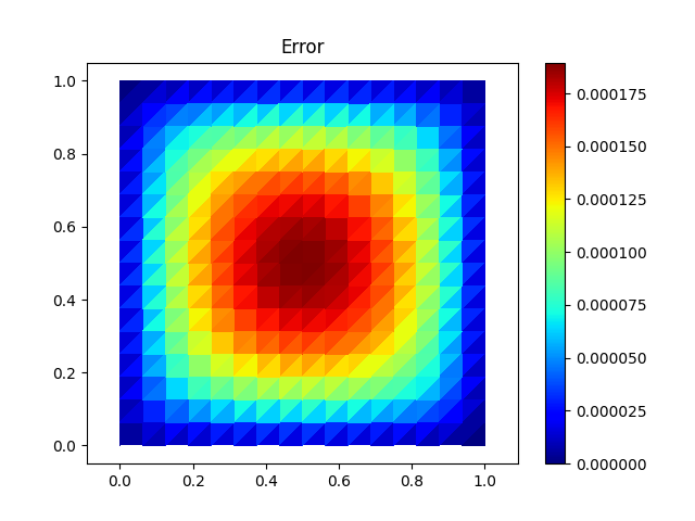
<matplotlib.collections.PolyCollection object at 0x7f71eb7e6990>

Norms and inner products

Finally, we want to check that we actually solved the system by computing \(\ell^2\) residual errors.

print('Residual error 1st solve: ', (b1-laplacian*u1).norm())
print('Residual error 2nd solve: ', (b2-laplacian*u2).norm())

Residual error 1st solve:  3.1227072320037345e-16
Residual error 2nd solve:  5.3146160357509636e-09

We observe that the first solution is accurate up to machine epsilon, and that the second solution satisfies the tolerance that we specified earlier.

We also compute errors in \(H^1_0\) and \(L^2\) norms. In order to compute the \(L^2\) error we need to assemble the mass matrix

\[\int_\Omega u v.\]

For the \(H^1_0\) error we can reuse the stiffness matrix that we assembled earlier.

mass = dm.assembleMass()

from numpy import sqrt

H10_error_1 = sqrt(b1.inner(u_interp_1-u1))
L2_error_1 = sqrt((u_interp_1-u1).inner(mass*(u_interp_1-u1)))
H10_error_2 = sqrt(b2.inner(u_interp_2-u2))
L2_error_2 = sqrt((u_interp_2-u2).inner(mass*(u_interp_2-u2)))

print('1st problem - H10:', H10_error_1, 'L2:', L2_error_1)
print('2nd problem - H10:', H10_error_2, 'L2:', L2_error_2)

1st problem - H10: 0.008458048434239385 L2: 0.00010638726221991537
2nd problem - H10: 0.125510275696724 L2: 0.0016209200215763343

This concludes our first example. Next, we turn to nonlocal equations.

plt.show()