Dirichlet condition for infinite horizon kernel

The following example can be found at examples/example_InfHorizonDirichlet.py in the PyNucleus repository.

We want to solve a problem with infinite horizon fractional kernel

\[\gamma(x,y) = \frac{c}{|x-y|^{d+2s}},\]

where \(c\) is the usual normalization constant, and imposes an inhomogeneous Dirichlet volume condition. We will have to make some assumption on the volume condition in order to make it computationally tractable. Here we assume that it is zero at some distance away from the domain.

\[\begin{split}(-\Delta)^s u &= f &&~in~ \Omega:=B_{1/2}(0),\\ u &= g &&~in~ \Omega_\mathcal{I}:=B_{1}(0)\setminus B_{1/2}(0), \\ u &= 0 &&~in~ \mathbb{R}^d \setminus B_{1}(0),\end{split}\]

where \(f\equiv 1\) and \(g\) is chosen to match the known exact solution \(u(x)=C(1-|x|^2)_+^s\) with some constant \(C\).

import numpy as np
import matplotlib.pyplot as plt
from PyNucleus import meshFactory, dofmapFactory, kernelFactory, functionFactory, solverFactory

Construct a mesh for \(\Omega\cup \Omega_\mathcal{I}\) and set up degree of freedom maps on \(\Omega\) and \(\Omega_\mathcal{I}\).

radius = 1.0
mesh = meshFactory('disc', n=8, radius=radius)
for _ in range(4):
    mesh = mesh.refine()

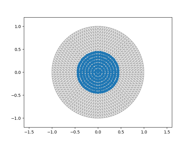
Get an indicator function for \(\Omega\). Subtract 1e-6 to avoid roundoff errors for nodes that are exactly on \(|x| = 0.5\).

OmegaIndicator = functionFactory('radialIndicator', 0.5*radius-1e-6)
dm = dofmapFactory('P1', mesh, OmegaIndicator)
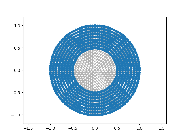
dmBC = dm.getComplementDoFMap()

plt.figure()
dm.plot(printDoFIndices=False)
plt.figure()
dmBC.plot(printDoFIndices=False)

• 
• 

Set up the kernel, rhs and known solution.

s = 0.75
kernel = kernelFactory('fractional', dim=mesh.dim, s=s, horizon=np.inf)
rhs = functionFactory('constant', 1.)
uex = functionFactory('solFractional', dim=mesh.dim, s=s, radius=radius)

Assemble the linear system

\[\begin{split}A_{\Omega,\Omega} u_{\Omega} + A_{\Omega,\Omega_\mathcal{I}} u_{\Omega_\mathcal{I}} &= f \\ u_{\Omega_\mathcal{I}} &= g\end{split}\]

Set up a solver for \(A_{\Omega,\Omega}\).

A_OmegaOmega = dm.assembleNonlocal(kernel, matrixFormat='H2')
A_OmegaOmegaI = dm.assembleNonlocal(kernel, dm2=dmBC)
f = dm.assembleRHS(rhs)
g = g = dmBC.interpolate(uex)
solver = solverFactory('lu', A=A_OmegaOmega, setup=True)

Efficiency of assembly with 2 DoFMaps is bad.

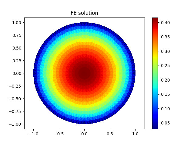
Compute FE solution and error between FE solution and interpolation of analytic expression

u_Omega = dm.zeros()
solver(f-A_OmegaOmegaI*g, u_Omega)
u = u_Omega.augmentWithBoundaryData(g)
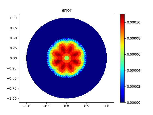
err = u.dm.interpolate(uex) - u

Plot FE solution and error

plt.figure()
plt.title('FE solution')
u.plot(flat=True)
plt.figure()
plt.title('error')
err.plot(flat=True)

• 
• 

<matplotlib.collections.PolyCollection object at 0x7f71eb794150>