Neumann condition for finite horizon kernel

The following example can be found at examples/example_Neumann.py in the PyNucleus repository.

$$\gamma (x,y)=c(\delta ){\chi }_{B_{\delta }(x)}(y),$$

where $c(\delta )$ is the usual normalization constant.

$$\begin{array}{rlrl}{\int }_{\mathrm{\Omega }\cup {\mathrm{\Omega }}_{\mathcal{I}}}(u(x)-u(y))\gamma (x,y)& =f(x)& & in\mathrm{\Omega }:=B_1(0),\\ {\int }_{\mathrm{\Omega }\cup {\mathrm{\Omega }}_{\mathcal{I}}}(u(x)-u(y))\gamma (x,y)& =g(x)& & in{\mathrm{\Omega }}_{\mathcal{I}}:=B_{1+\delta }(0)\setminus B_1(0),\end{array}$$

where $f\equiv 2$ and

$$g(x)=c(\delta )[|x|((1+\delta -|x|{)}^2-{\delta }^2)+\frac{1}{3}((1+\delta -|x|{)}^3+{\delta }^3)].$$

The exact solution is $u(x)=C-x^2$ where $C$ is an arbitrary constant.

import numpy as np
import matplotlib.pyplot as plt
from PyNucleus import (nonlocalMeshFactory, dofmapFactory, kernelFactory,
                       functionFactory, solverFactory, NEUMANN, NO_BOUNDARY)
from PyNucleus_base.linear_operators import Dense_LinearOperator

Set up kernel, load $f$, the analytic solution and the flux data $g$.

kernel = kernelFactory('constant', dim=1, horizon=0.4)
load = functionFactory('constant', 2.)
analyticSolution = functionFactory('Lambda', lambda x: -x[0]**2)

def fluxFun(x):
    horizon = kernel.horizonValue
    dist = 1+horizon-abs(x[0])
    assert dist >= 0
    return 2*kernel.scalingValue * (abs(x[0]) * (dist**2-horizon**2) + 1./3. * (dist**3+horizon**3))

flux = functionFactory('Lambda', fluxFun)

Construct a degree of freedom map for the entire mesh

mesh, nI = nonlocalMeshFactory('interval', kernel=kernel, boundaryCondition=NEUMANN)
for _ in range(3):
    mesh = mesh.refine()

dm = dofmapFactory('P1', mesh, NO_BOUNDARY)
dm

P1 DoFMap with 57 DoFs and 0 boundary DoFs.

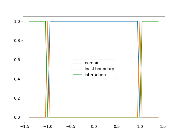
The second return value of the nonlocal mesh factory contains indicator functions:

dm.interpolate(nI['domain']).plot(label='domain')
dm.interpolate(nI['boundary']).plot(label='local boundary')
dm.interpolate(nI['interaction']).plot(label='interaction')
plt.legend()

<matplotlib.legend.Legend object at 0x7fbee00cf380>

Assemble the RHS vector by using the load on the domain $\mathrm{\Omega }$ and the flux function on the interaction domain ${\mathrm{\Omega }}_{\mathcal{I}}$

A = dm.assembleNonlocal(kernel)
b = dm.assembleRHS(load*nI['domain'] + flux*(nI['interaction']+nI['boundary']))

Solve the linear system. Since it is singular (shifts by a constant form the nullspace) we augment the system and then project out the zero mode.

u = dm.zeros()

Augment the system

correction = Dense_LinearOperator(np.ones(A.shape))
solver = solverFactory('lu', A=A+correction, setup=True)
solver(b, u)

1

project out the nullspace component

const = dm.ones()
u = u - (u.inner(const)/const.inner(const))*const

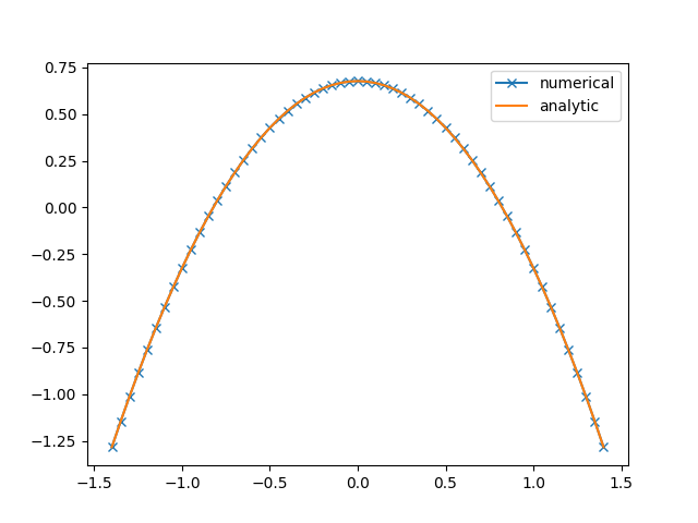
Interpolate the exact solution and project out zero mode as well.

uex = dm.interpolate(analyticSolution)
uex = uex - (uex.inner(const)/const.inner(const))*const

u.plot(label='numerical', marker='x')
uex.plot(label='analytic')
plt.legend()

<matplotlib.legend.Legend object at 0x7fbedfcdc910>