Nonlocal problems

I this second example, we will assemble and solve several nonlocal equations. The full code of this example can be found in examples/example_nonlocal.py in the PyNucleus repository.

PyNucleus can assemble operators of the form

\[\mathcal{L}u(x) = \operatorname{p.v.} \int_{\mathbb{R}^d} [u(y)-u(x)] \gamma(x, y) dy.\]

The kernel \(\gamma\) is of the form

\[\gamma(x,y) = \frac{\phi(x, y)}{|x-y|^{\beta(x,y)}} \chi_{\mathcal{N}(x)}(y).\]

Here, \(\phi\) is a positive function, and \(\chi\) is the indicator function. The interaction neighborhood \(\mathcal{N}(x) \subset \mathbb{R}^d\) is often given as parametrized by the so-called horizon \(0<\delta\le\infty\):

\[\mathcal{N}(x) = \{y \in \mathbb{R}^d \text{ such that } ||x-y||_p<\delta\}.\]

where \(p \in \{1,2,\infty\}\). Other types of neighborhoods are also possible.

The singularity \(\beta\) of the kernel crucially influences properties of the kernel:

• fractional type: \(\beta(x,y)=d+2s(x,y)\), where \(d\) is the spatial dimension and \(s(x,y)\) is the fractional order.

• constant type \(\beta(x,y)=0\)

• peridynamic type \(\beta(x,y)=1\)

A fractional kernel

We start off by creating a fractional kernel with infinite horizon and constant fractional order \(s=0.75\).

import matplotlib.pyplot as plt
from time import time
from PyNucleus import kernelFactory
print(kernelFactory)

Available:
'fractional', signature: '(dim, s, horizon=None, interaction=None, scaling=None, normalized=True, piecewise=True, phi=None, boundary=False, derivative=0, tempered=0.0, max_horizon=nan)'
'indicator' with aliases ['constant'], signature: '(dim, kernel, horizon, scaling=None, interaction=None, normalized=True, piecewise=True, phi=None, boundary=False, monomialPower=nan, variance=1.0, exponentialRate=1.0, a=1.0, max_horizon=nan)'
'inverseDistance' with aliases ['peridynamic', 'inverseOfDistance'], signature: '(dim, kernel, horizon, scaling=None, interaction=None, normalized=True, piecewise=True, phi=None, boundary=False, monomialPower=nan, variance=1.0, exponentialRate=1.0, a=1.0, max_horizon=nan)'
'gaussian', signature: '(dim, kernel, horizon, scaling=None, interaction=None, normalized=True, piecewise=True, phi=None, boundary=False, monomialPower=nan, variance=1.0, exponentialRate=1.0, a=1.0, max_horizon=nan)'
'exponential', signature: '(dim, kernel, horizon, scaling=None, interaction=None, normalized=True, piecewise=True, phi=None, boundary=False, monomialPower=nan, variance=1.0, exponentialRate=1.0, a=1.0, max_horizon=nan)'
'polynomial', signature: '(dim, kernel, horizon, scaling=None, interaction=None, normalized=True, piecewise=True, phi=None, boundary=False, monomialPower=nan, variance=1.0, exponentialRate=1.0, a=1.0, max_horizon=nan)'
'logInverseDistance', signature: '(dim, kernel, horizon, scaling=None, interaction=None, normalized=True, piecewise=True, phi=None, boundary=False, monomialPower=nan, variance=1.0, exponentialRate=1.0, a=1.0, max_horizon=nan)'
'monomial', signature: '(dim, kernel, horizon, scaling=None, interaction=None, normalized=True, piecewise=True, phi=None, boundary=False, monomialPower=nan, variance=1.0, exponentialRate=1.0, a=1.0, max_horizon=nan)'

from numpy import inf

kernelFracInf = kernelFactory('fractional', dim=2, s=0.75, horizon=inf)
print(kernelFracInf)

kernel(fractional, 0.75, R^2, constantFractionalLaplacianScaling(0.75,inf -> 0.08558356484527617))

plt.figure().gca().set_title('Fractional kernel')
kernelFracInf.plot()

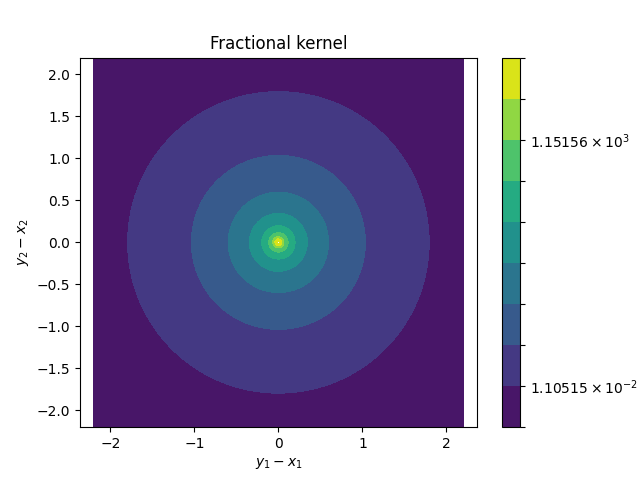
By default, kernels are normalized so that their local limits recover the classical Laplacian. This can be disabled by passing normalized=False.

Nonlocal assembly

We will be solving the problem

\[\begin{split}-\mathcal{L} u &= f && \text{ in } \Omega=B(0,1)\subset\mathbb{R}^2, \\ u &= 0 && \text{ in } \mathbb{R}^2 \setminus \Omega,\end{split}\]

for constant forcing function \(f=1\).

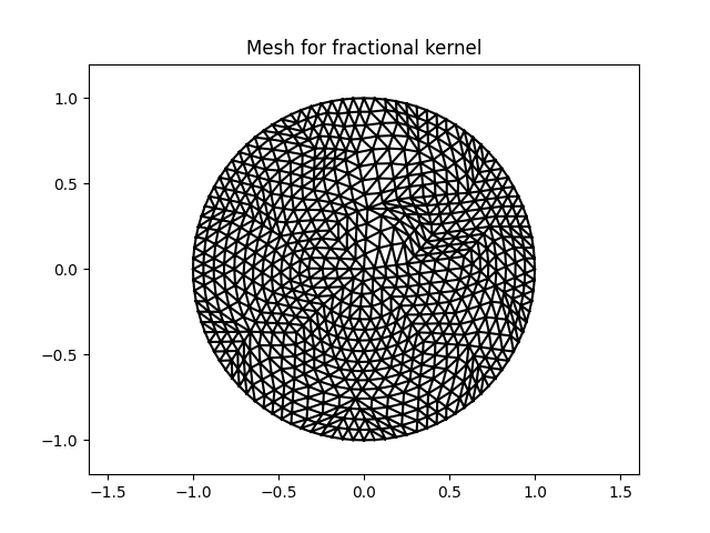
First, we generate a mesh. Instead of the meshFactory used in the previous example, we now use the nonlocalMeshFactory. The advantage is that this factory can generate meshes with appropriate interaction domains. For this particular example, the factory will not generate any interaction domain, since the homogeneous Dirichlet condition on \(\mathbb{R}^2\setminus\Omega\) can be enforced via a boundary integral.

from PyNucleus import nonlocalMeshFactory, HOMOGENEOUS_DIRICHLET

# Get a mesh that is appropriate for the problem, i.e. with the required interaction domain.
meshFracInf, _ = nonlocalMeshFactory('disc', kernel=kernelFracInf, boundaryCondition=HOMOGENEOUS_DIRICHLET, hTarget=0.15)

print(meshFracInf)

mesh2d with 763 vertices and 1,424 cells

plt.figure().gca().set_title('Mesh for fractional kernel')
meshFracInf.plot()

Next, we obtain a piecewise linear, continuous DoFMap on the mesh, assemble the RHS and interpolate the known analytic solution. We assemble the nonlocal operator by passing the kernel to the assembleNonlocal method of the DoFMap object. The optional parameter matrixFormat determines what kind of linear operator is assembled. We time the assembly of the operator as a dense matrix, and as a hierarchical matrix, and inspect the resulting objects.

from PyNucleus import dofmapFactory, functionFactory

dmFracInf = dofmapFactory('P1', meshFracInf)

rhs = functionFactory('constant', 1.)
exact_solution = functionFactory('solFractional', dim=2, s=0.75)

b = dmFracInf.assembleRHS(rhs)
u_exact = dmFracInf.interpolate(exact_solution)
u = dmFracInf.zeros()

We assemble the operator in dense format.

start = time()
A_fracInf = dmFracInf.assembleNonlocal(kernelFracInf, matrixFormat='dense')

print('Dense assembly took {}s'.format(time()-start))
print(A_fracInf)
print("Memory size: {} KB".format(A_fracInf.getMemorySize() >> 10))

Dense assembly took 2.4222586154937744s
<663x663 Dense_LinearOperator>
Memory size: 3434 KB

Then we assemble the operator in hierarchical matrix format.

start = time()
A_fracInf_h2 = dmFracInf.assembleNonlocal(kernelFracInf, matrixFormat='h2')

print('Hierarchical assembly took {}s'.format(time()-start))
print(A_fracInf_h2)
print("Memory size: {} KB".format(A_fracInf_h2.getMemorySize() >> 10))

Hierarchical assembly took 2.608210325241089s
<663x663 H2Matrix 0.374045 fill from near field, 0.123774 fill from tree, 0.206848 fill from clusters, 63 tree nodes, 186 far-field cluster pairs>
Memory size: 2419 KB

It can be observed that both assembly routines take roughly the same amount of time. The reason for this is that the operator itself has quite small dimensions. For larger number of unknowns, we expect the hierarchical assembly scale like \(\mathcal{O}(N \log^{2d} N)\), whereas the dense assembly will scale at best like \(\mathcal{O}(N^2)\). The memory usage of the hierarchical matrix is slightly better and scales similar to the complexity of assembly.

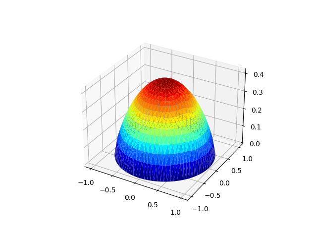
Similar to the local PDE example, we can then solve the resulting linear equation and compute the error in energy norm.

from PyNucleus import solverFactory
from numpy import sqrt

solver = solverFactory('lu', A=A_fracInf, setup=True)
solver(b, u)

Hs_err = sqrt(abs(b.inner(u-u_exact)))

print('Hs error: {}'.format(Hs_err))

Hs error: 0.05503838572322174

plt.figure().gca().set_title('Numerical solution, fractional kernel')
u.plot()

<Axes3D: >

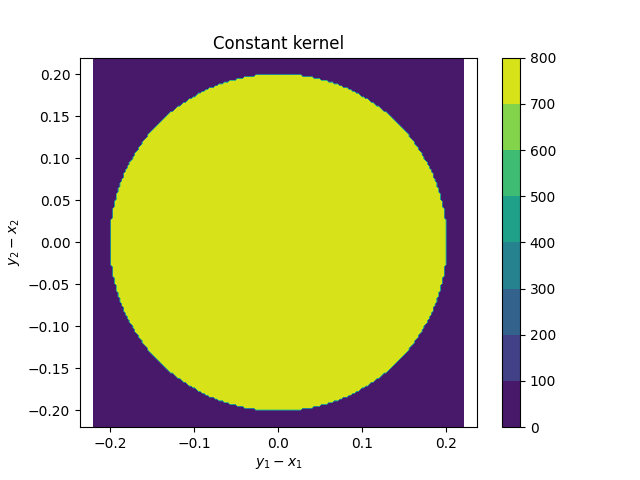
A finite horizon case with Dirichlet volume condition

Next, we solve a nonlocal Poisson problem involving a constant kernel with finite horizon. We will choose \(\gamma(x,y) \sim \chi_{\mathcal{N}(x)}(y)\) for a neighborhood defined by the 2-norm and horizon \(\delta=0.2\), and solve

\[\begin{split}-\mathcal{L} u &= f && \text{ in } \Omega=[0,1]^2, \\ u &= -(x_1^2 + x_2^2)/4 && \text{ in } \mathcal{I},\end{split}\]

where the interaction domain is given by

\[\mathcal{I} := \{y\in\mathbb{R}^2\setminus\Omega \text{ such that } \exists x\in\Omega: \gamma(x,y)\neq 0\}.\]

kernelConst = kernelFactory('constant', dim=2, horizon=0.2)
print(kernelConst)

Kernel(indicator, |x-y|_2 <= 0.2, constantIntegrableScaling(0.2 -> 795.7747154594766))

plt.figure().gca().set_title('Constant kernel')
kernelConst.plot()

from PyNucleus import DIRICHLET

meshConst, nIConst = nonlocalMeshFactory('square', kernel=kernelConst, boundaryCondition=DIRICHLET, hTarget=0.18)

print(meshConst)
print(nIConst)

mesh2d with 569 vertices and 1,056 cells
{'domain': squareIndicator, 'boundary': 1.0*1.0*1.0+-1.0*squareIndicator+-1.0*1.0*1.0+-1.0*squareIndicator, 'interaction': 1.0*1.0+-1.0*squareIndicator, 'tag': -128, 'zeroExterior': False}

The dictionary nIConst contains several indicator functions that we will use to distinguish between interior and interaction domain.

plt.figure().gca().set_title('Mesh for constant kernel')
meshConst.plot()

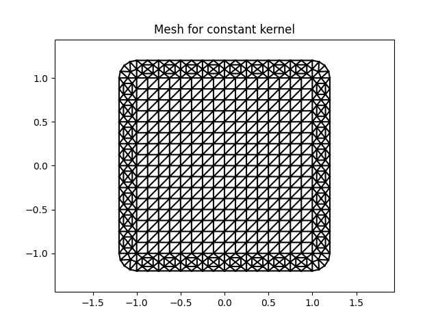
We can observe that the nonlocalMeshFactory generated a mesh that includes the interaction domain.

We set up 2 DoFMaps this time, one for the unknown interior degrees of freedom and one for the Dirichlet volume condition.

dmConst = dofmapFactory('P1', meshConst, nIConst['domain'])
dmConstInteraction = dmConst.getComplementDoFMap()

print(dmConst)
print(dmConstInteraction)

P1 DoFMap with 225 DoFs and 344 boundary DoFs.
P1 DoFMap with 344 DoFs and 225 boundary DoFs.

We can see that they are complementary to each other. Next, we assemble two matrices.

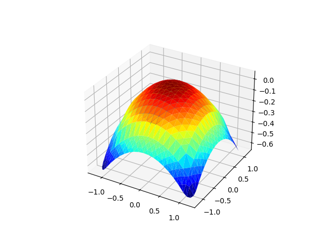
A_const = dmConst.assembleNonlocal(kernelConst, matrixFormat='sparse')
B_const = dmConst.assembleNonlocal(kernelConst, dm2=dmConstInteraction, matrixFormat='sparse')

g = functionFactory('Lambda', lambda x: -(x[0]**2 + x[1]**2)/4)
g_interp = dmConstInteraction.interpolate(g)

b = dmConst.assembleRHS(rhs)-(B_const*g_interp)
u = dmConst.zeros()

solver = solverFactory('cg', A=A_const, setup=True)
solver.maxIter = 1000
solver.tolerance = 1e-8

solver(b, u)

u_global = u.augmentWithBoundaryData(g_interp)

plt.figure().gca().set_title('Numerical solution, constant kernel')
u_global.plot()

<Axes3D: >

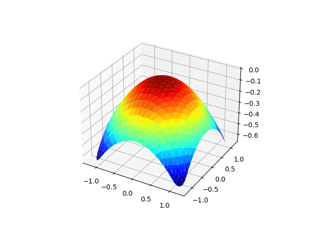
plt.figure().gca().set_title('Analytic solution, constant kernel')
u_global.dm.interpolate(g).plot()

<Axes3D: >

print(A_const)

<225x225 SSS_LinearOperator with 4437 stored elements>

plt.show()
# sphinx_gallery_thumbnail_number = 3