Operator interpolation

This example demostrates the construction of a family of fractional Laplacians parametrized by the fractional order using operator interpolation. This can reduce the cost compared to assembling a new matrix for each value.

The fractional Laplacian

\[(-\Delta)^{s} \text{ for } s \in [s_{\min}, s_{\max}] \subset (0, 1)\]

is approximated by

\[(-\Delta)^{s} \approx \sum_{m=0}^{M} \Theta_{k,m}(s) (-\Delta)^{s_{k,m}} \text{ for } s \in \mathcal{S}_{k}\]

for a sequence of intervals \(\mathcal{S}_{k}\) that cover \([s_{\min}, s_{\max}]\) and scalar coefficients \(\Theta_{k,m}(s)\). The number of intervals and interpolation nodes is picked so that the interpolation error is dominated by the discretization error.

The following example can be found at examples/example_operator_interpolation.py in the PyNucleus repository.

import logging
from PyNucleus_base.utilsFem import TimerManager
import numpy as np
import matplotlib.pyplot as plt

fmt = '{message}'
logging.basicConfig(level=logging.INFO,
                    format=fmt,
                    style='{',
                    datefmt="%Y-%m-%d %H:%M:%S")
logger = logging.getLogger('__main__')
timer = TimerManager(logger)

We set up a mesh, a dofmap and a fractional kernel. Instead of specifying a single value for the fractional order, we allow a range of values \([s_{\min}, s_{\max}]=[0.05, 0.95]\).

from PyNucleus import meshFactory, dofmapFactory, kernelFactory, functionFactory, solverFactory
from PyNucleus_nl.operatorInterpolation import admissibleSet

# Set up a mesh and a dofmap on it.
mesh = meshFactory('interval', hTarget=2e-3, a=-1, b=1)
dm = dofmapFactory('P1', mesh)

# Construct a RHS vector and a vector for the solution.
f = functionFactory('constant', 1.)
b = dm.assembleRHS(f)
u = dm.zeros()

# construct a fractional kernel with fractional order in S = [0.05, 0.95]
s = admissibleSet([0.05, 0.95])
kernel = kernelFactory('fractional', s=s, dim=mesh.dim)

Next, we call the assembly of a nonlocal operator as before. The operator is set up to be constructed on-demand. We partition the interval S into several sub-interval and construct a Chebyshev interpolant on each sub-interval. Therefore this operation is fast.

with timer('operator creation'):
    A = dm.assembleNonlocal(kernel, matrixFormat='H2')

operator creation in 0.123 s

Next, we choose the value of the fractional order. This needs to be within the range that we specified earlier. We set s = 0.75.

A.set(0.75)

Let’s solve a system. This triggers the assembly of the operators for the matrices at the interpolation nodes of the interval that contains s. The required matrices are constructed on-demand and then stay in memory.

with timer('solve 1 (slow)'):
    solver = solverFactory('cg-jacobi', A=A, setup=True)
    solver.maxIter = 1000
    numIter = solver(b, u)
logger.info('Solved problem for s={} in {} iterations (residual norm {})'.format(A.get(), numIter, solver.residuals[-1]))

solve 1 (slow) in 0.6 s
Solved problem for s=0.75 in 181 iterations (residual norm 9.1977050437471e-06)

This solve is relatively slow, as it involves the assembly of the nonlocal operators that are needed for the interpolation. We select a different value for the fractional order that is close to the first. Solving a linear system with this value is faster as we have already assembled the operator needed for the interpolation.

with timer('solve 2 (fast)'):
    A.set(0.76)
    solver = solverFactory('cg-jacobi', A=A, setup=True)
    solver.maxIter = 1000
    numIter = solver(b, u)
logger.info('Solved problem for s={} in {} iterations (residual norm {})'.format(A.get(), numIter, solver.residuals[-1]))

solve 2 (fast) in 0.135 s
Solved problem for s=0.76 in 190 iterations (residual norm 8.897510981001526e-06)

Next, we save the operator to file. This first triggers the assembly of all operators nescessary to represent every value in \(s\in[0.05,0.95]\).

import h5py

with timer('save operator'):
    h5_file = h5py.File('test.hdf5', 'w')
    A.HDF5write(h5_file.create_group('A'))
    dm.HDF5write(h5_file.create_group('dm'))
    h5_file.close()

save operator in 17.5 s

Next, we read the operator back in.

from PyNucleus_base.linear_operators import LinearOperator
from PyNucleus_fem.DoFMaps import DoFMap

with timer('load operator'):
    h5_file = h5py.File('test.hdf5', 'r')
    A_2 = LinearOperator.HDF5read(h5_file['A'])
    dm_2 = DoFMap.HDF5read(h5_file['dm'])
    h5_file.close()

/home/runner/work/PyNucleus/PyNucleus/examples/example_operator_interpolation.py:125: DeprecationWarning: __array__ implementation doesn't accept a copy keyword, so passing copy=False failed. __array__ must implement 'dtype' and 'copy' keyword arguments.
  A_2 = LinearOperator.HDF5read(h5_file['A'])
/home/runner/work/PyNucleus/PyNucleus/examples/example_operator_interpolation.py:126: DeprecationWarning: __array__ implementation doesn't accept a copy keyword, so passing copy=False failed. __array__ must implement 'dtype' and 'copy' keyword arguments.
  dm_2 = DoFMap.HDF5read(h5_file['dm'])
load operator in 5.62 s

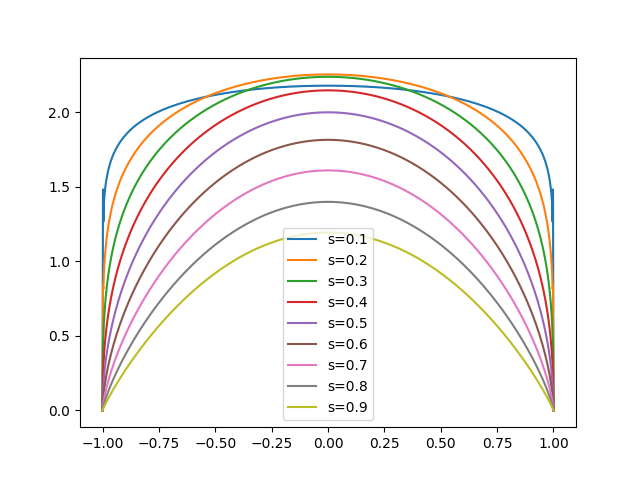
Finally, we set up and solve a series of linear systems with the operator we loaded.

f_2 = functionFactory('constant', 2.)
b_2 = dm_2.assembleRHS(f_2)
for sVal in np.linspace(0.1, 0.9, 9):
    with timer('solve 3 (fast)'):
        u_2 = dm_2.zeros()
        A_2.set(sVal)
        solver = solverFactory('cg-jacobi', A=A_2, setup=True)
        solver.maxIter = 1000
        numIter = solver(b_2, u_2)
    logger.info('Solved problem for s={:.1} in {} iterations (residual norm {})'.format(A_2.get(), numIter, solver.residuals[-1]))
    u_2.plot(label='s={:.1}'.format(sVal))
plt.legend()

solve 3 (fast) in 0.00655 s
Solved problem for s=0.1 in 7 iterations (residual norm 3.3399038658481357e-06)
solve 3 (fast) in 0.0108 s
Solved problem for s=0.2 in 13 iterations (residual norm 3.661677431067543e-06)
solve 3 (fast) in 0.0163 s
Solved problem for s=0.3 in 21 iterations (residual norm 7.068770471207567e-06)
solve 3 (fast) in 0.0249 s
Solved problem for s=0.4 in 34 iterations (residual norm 8.650357989614632e-06)
solve 3 (fast) in 0.04 s
Solved problem for s=0.5 in 55 iterations (residual norm 9.299204350465222e-06)
solve 3 (fast) in 0.0666 s
Solved problem for s=0.6 in 90 iterations (residual norm 8.670054190291985e-06)
solve 3 (fast) in 0.105 s
Solved problem for s=0.7 in 146 iterations (residual norm 9.855504121489942e-06)
solve 3 (fast) in 0.171 s
Solved problem for s=0.8 in 234 iterations (residual norm 8.647867737473381e-06)
solve 3 (fast) in 0.253 s
Solved problem for s=0.9 in 361 iterations (residual norm 9.690893462011102e-06)

<matplotlib.legend.Legend object at 0x7f71f1bfbf90>

plt.show()