Shapes

Shape information is very important in Structural Dynamics. In general, a shape is a specific deformation pattern of a structure, whether it is at a specific instance in time or specific frequency line (which we generally refer to as a deflection shape) or whether it is the shape associated with a specific mode of the structure (which we generally refer to as a mode shape). SDynPy tracks these deflections and associates them with coordinates as described in the previous documentation page. Shapes in SDynPy also integrate very well with geometry in SDynPy, allowing for quick visualization of the shape in an interactive, 3D sense.

This document will demonstrate how shapes are defined and used in SDynPy. We will start by defining the shape object, then walk through different use-cases in SDynPy.

Let’s import SDynPy and start looking at shapes!

import sdynpy as sdpy
import numpy as np

SDynPy Shape Objects

In SDynPy, the object used to represent mode shapes or deflection shapes is the ShapeArray. As the name implies, this is a SdynpyArray subclass and therefore has all of the functionality of the SdynpyArray and the NumPy ndarray.

Being able to represent both mode shapes and deflection shapes, ShapeArray objects have two types. They can be “real” shapes, meaning the shape matrix is entirely composed of real numbers, or they can be “complex” shapes, meaning the shape matrix contains complex numbers. These correspond to real and complex modes, respectively. Different types of deflection shapes may also be real or complex depending on their source. For example, a frequency line in a frequency response function is a complex shape. A single time instance in a deflection time history would be a real shape.

Similar to other SdynpyArray subclasses, there is a function shape_array to help us construct ShapeArray objects that uses the same name except with snake_case capitalization instead of CamelCase. Let’s construct a sample ShapeArray so we can investigate it more thoroughly.

# Set up some initial sizes
num_shapes = 10
num_coords = 3

# Create a shape with random data in its fields
shapes = sdpy.shape_array(
    coordinate = sdpy.coordinate_array(np.arange(num_coords)+1,'X+'),
    shape_matrix = np.random.randn(num_shapes,num_coords),
    frequency = np.arange(num_shapes),
    damping = np.arange(num_shapes)/100, # /100 is converting from percent to fraction
    modal_mass = np.arange(num_shapes),
    comment1 = [f'Comment1: Shape {i}' for i in range(num_shapes)],
    comment2 = [f'Comment2: Shape {i}' for i in range(num_shapes)],
    comment3 = [f'Comment3: Shape {i}' for i in range(num_shapes)],
    comment4 = [f'Comment4: Shape {i}' for i in range(num_shapes)],
    comment5 = [f'Comment5: Shape {i}' for i in range(num_shapes)])

Note that when we create a ShapeArray object, we must define the coordinates of each of the shape coefficients with a CoordinateArray. This allows SDynPy to track which coordinates correspond to which coefficients, and enables SDynPy to handle some of the bookkeeping for us. We can also assign frequency, damping, and modal mass corresponding to each shape, as well as up to five comments for each shape. These comments may be used to store, for example, a description of the mode shape (e.g. “First Bending in the X direction”) or any other pertinent information regarding the shape.

Now that we have a ShapeArray defined, let’s look at some of its fields and dtype.

shapes.fields

('frequency',
 'damping',
 'coordinate',
 'shape_matrix',
 'modal_mass',
 'comment1',
 'comment2',
 'comment3',
 'comment4',
 'comment5')

shapes.dtype

dtype([('frequency', '<f8'), ('damping', '<f8'), ('coordinate', [('node', '<u8'), ('direction', 'i1')], (3,)), ('shape_matrix', '<f8', (3,)), ('modal_mass', '<f8'), ('comment1', '<U80'), ('comment2', '<U80'), ('comment3', '<U80'), ('comment4', '<U80'), ('comment5', '<U80')])

We can see that for each shape, we have floating point fields frequency, damping, and modal_mass. In SDynPy, the convention is to have the frequency be in “cycles per time” (e.g. Hz) as opposed to angle per time (e.g. rad/s). SDynPy also treats the damping value as the “fraction of critical damping”, so a damping value of 1 would be equivalent to 100% of critical damping, i.e. a critically damped structure. A damping of 0.05 would be 5% critical damping, etc. Modal mass can also be defined, but if we scale shapes to be mass-normalized, this value is typically 1.

We also see that we have the 5 comment fields, comment1 through comment5. The choice of 5 comment fields stems from the Universal File Format Dataset 55, which is used to store “data at nodes”, also known as shapes. Dataset 55 also stores 5 comments associated with each shape, and SDynPy objects typically try to match the corresponding Universal File Format object.

The last two fields shape_matrix and coordinate each have a dtype with shape (3,), meaning that each shape in the ShapeArray object has three shape coefficients and three coordinates associated with it. The shape coefficients are stored in the current ShapeArray objects as floating point numbers. The coordinate field actually has a compound dtype, wich node and direction fields. Readers having just read the Complex Modes page will recognize this as the dtype of the CoordinateArray object, meaning ShapeArray objects store coordinate information as a CoordinateArray.

shapes.dtype['coordinate']

dtype(([('node', '<u8'), ('direction', 'i1')], (3,)))

# Create a dummy coordinate array so we can see its dtype
sdpy.coordinate_array(1,1).dtype

dtype([('node', '<u8'), ('direction', 'i1')])

Indeed, if we request the coordinate field of the ShapeArray object, we will receive a CoordinateArray object.

shapes.coordinate

coordinate_array(string_array=
array([['1X+', '2X+', '3X+'],
       ['1X+', '2X+', '3X+'],
       ['1X+', '2X+', '3X+'],
       ['1X+', '2X+', '3X+'],
       ['1X+', '2X+', '3X+'],
       ['1X+', '2X+', '3X+'],
       ['1X+', '2X+', '3X+'],
       ['1X+', '2X+', '3X+'],
       ['1X+', '2X+', '3X+'],
       ['1X+', '2X+', '3X+']], dtype='<U3'))

The shape_matrix once again holds the shape coefficients. It has a shape of (3,), meaning there are three coefficients for each shape. Recall, however, that when a NumPy ndarray has a field with a dtype containing a shape, the shape of that dtype is appended to the shape of the array itself when requesting the field. For example, we currently have 10 shapes in our ShapeArray object.

shapes.shape

(10,)

With each shape having 3 coordinates, the shape of the shape_matrix field is then (10,3).

shapes.shape_matrix.shape

(10, 3)

Users familiar with structural dynamics may question the shape of this shape_array matrix; the usual mode shape matrix will have a number of rows equal to the number of degrees of freedom, and a number of columns equal to the number of modes of the system. Here we have the transpose of that definition. However, this design decision was made because it allows ShapeArray objects to fit well into the NumPy ndarray object from which it inherits. For example, it allows us to elegantly generalize to multidimensional ShapeArray objects.

nd_shapes = shapes.reshape(5,2)
nd_shapes.shape

(5, 2)

With a multidimensional ShapeArray object, all the shape dimensions are on the left, and the coordinate dimensions are on the right in the shape_matrix field. For example, in this case we have a shape (5,2) ShapeArray and a shape (3,) number of coordinates, so we will have a shape (5,2,3) shape matrix.

nd_shapes.shape_matrix.shape

(5, 2, 3)

If we imagine trying to treat the shape_matrix as the traditional mode shape matrix, it would involve the first however many dimensions as shape dimensions, than the second to last dimension as a coordinate dimension, then the last dimension as a shape dimension again, which is needlessly confusing. Users new to NumPy or SDynPy may wonder why we would ever need to have a multidimensional ShapeArray. However, once users understand the power of broadcasting NumPy arrays, they will see many use cases for multidimensional arrays. For example, perhaps the user is trying to compare a set of modes from a test with a set of modes from an analysis. The user may structure the modes in a 2D ShapeArray object, with the first dimension representing test or analysis and the second dimension representing the mode number. For-looping over the transpose of this ShapeArray would then peel off pairs of test and analysis modes.

The author of SDynPy does, however, recognize the potentially confusing aspect, so users looking for a field like the shape_matrix but with the dimension ordering of a mode shape matrix can see the modeshape property.

shapes.modeshape.shape

(3, 10)

This property generally just transposes the last two dimension of the shape_matrix field. Therefore, if one does have a multidimensional ShapeArray, they will see that the first dimensions are unchanged. In the case of the nd_shapes ShapeArray, which was shape (5,2), the shape_matrix had shape (5,2,3). Transposing the last two dimensions to get the modeshape property will give a (5,3,2) array. The last two dimensions of the array are therefore treated as the mode shape matrix, which is consistent with NumPy’s typical matrix representation.

nd_shapes.shape_matrix.shape

(5, 2, 3)

nd_shapes.modeshape.shape

(5, 3, 2)

Note that the modeshape property is actually a view into the shape_matrix field. This means that if we modify the modeshape field in-place (e.g. by assigning to an index of it), then it will also change the shape_matrix field.

nd_shapes.modeshape[:] = np.array([[1],
                                   [2],
                                   [3]])

We can see that this has been broadcast out into the modeshape matrix:

nd_shapes.modeshape

array([[[1., 1.],
        [2., 2.],
        [3., 3.]],

       [[1., 1.],
        [2., 2.],
        [3., 3.]],

       [[1., 1.],
        [2., 2.],
        [3., 3.]],

       [[1., 1.],
        [2., 2.],
        [3., 3.]],

       [[1., 1.],
        [2., 2.],
        [3., 3.]]])

And indeed the shape_matrix is equivalent, but transposed.

nd_shapes.shape_matrix

array([[[1., 2., 3.],
        [1., 2., 3.]],

       [[1., 2., 3.],
        [1., 2., 3.]],

       [[1., 2., 3.],
        [1., 2., 3.]],

       [[1., 2., 3.],
        [1., 2., 3.]],

       [[1., 2., 3.],
        [1., 2., 3.]]])

If we type a ShapeArray variable name into the terminal, we get a tabular representation of the ShapeArray.

nd_shapes

   Index,  Frequency,    Damping,     # DoFs
  (0, 0),     0.0000,    0.0000%,          3
  (0, 1),     1.0000,    1.0000%,          3
  (1, 0),     2.0000,    2.0000%,          3
  (1, 1),     3.0000,    3.0000%,          3
  (2, 0),     4.0000,    4.0000%,          3
  (2, 1),     5.0000,    5.0000%,          3
  (3, 0),     6.0000,    6.0000%,          3
  (3, 1),     7.0000,    7.0000%,          3
  (4, 0),     8.0000,    8.0000%,          3
  (4, 1),     9.0000,    9.0000%,          3

Creating Shapes from Scratch

Now that we’ve discussed a bit about the ShapeArray object, let’s look more closely at how we can construct one. We will assume that our shapes are sines and cosines of increasing frequency. If we plot these shapes on a line, it might look a bit like a beam bending mode.

First, let’s create the shape coefficients. We can use NumPy to construct these quantities.

t = np.linspace(0,2*np.pi,50,endpoint=True)
freqs = (np.arange(5)+1)/2

# Use broadcasting to create the arguments easily
sines = np.sin(freqs[:,np.newaxis]*t)
cosines = np.cos(freqs[:,np.newaxis]*t)

To see what they look like, we can plot with Matplotlib.

import matplotlib.pyplot as plt

fig,axes = plt.subplots(len(freqs),2,
                        layout='constrained',
                        sharex=True,
                        sharey=True)

for ax_row, sine_function, cosine_function in zip(axes,sines,cosines):
    ax_row[0].plot(sine_function)
    ax_row[1].plot(cosine_function)

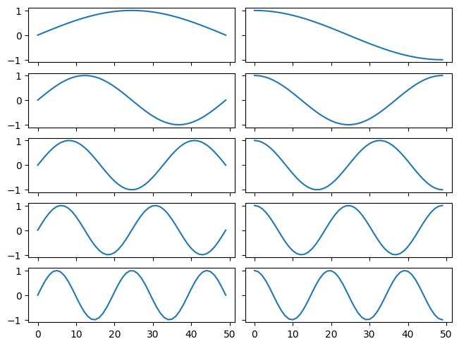
We have created both sine and cosine functions because we will be looking at both real and complex modes. Let’s now create the shape_matrix field. We see that our functions are already the correct shapes, as they have shape (5,50) or (num_shape, num_coord).

sines.shape

(5, 50)

cosines.shape

(5, 50)

We will assign the freqs quantity to the frequencies, and let the damping and modal mass be default values (0 and 1, respectively). We will also ignore comments for now.

We do, however, need to assign coordinates to the shape. The CoordinateArray we use will typically be in reference to some Geometry object. In our case, we do not have a Geometry defined yet, so we will simply assume the coordinates are nodes 1-50 in the \(Z+\) direction.

shape_coords = sdpy.coordinate_array(np.arange(50)+1, 'Z+')
shape_coords

coordinate_array(string_array=
array(['1Z+', '2Z+', '3Z+', '4Z+', '5Z+', '6Z+', '7Z+', '8Z+', '9Z+',
       '10Z+', '11Z+', '12Z+', '13Z+', '14Z+', '15Z+', '16Z+', '17Z+',
       '18Z+', '19Z+', '20Z+', '21Z+', '22Z+', '23Z+', '24Z+', '25Z+',
       '26Z+', '27Z+', '28Z+', '29Z+', '30Z+', '31Z+', '32Z+', '33Z+',
       '34Z+', '35Z+', '36Z+', '37Z+', '38Z+', '39Z+', '40Z+', '41Z+',
       '42Z+', '43Z+', '44Z+', '45Z+', '46Z+', '47Z+', '48Z+', '49Z+',
       '50Z+'], dtype='<U4'))

Now let’s create the ShapeArray object. We will create a set of “real” shapes with just the sines, and we will create a “complex” shapes with the sines as the real part and the cosines as the imaginary part.

real_shapes = sdpy.shape_array(
    coordinate = shape_coords,
    shape_matrix = sines,
    frequency = freqs)

complex_shapes = sdpy.shape_array(
    coordinate = shape_coords,
    shape_matrix = sines+1j*cosines,
    frequency = freqs)

Note that when we create objects using the shape_array method, the arguments broadcast to the correct size. For example, if we wanted to explicitly set the damping to 0 and the modal mass to 1, we could simply type:

real_shapes = sdpy.shape_array(
    coordinate = shape_coords,
    shape_matrix = sines,
    frequency = freqs,
    damping = 0,
    modal_mass = 1)

complex_shapes = sdpy.shape_array(
    coordinate = shape_coords,
    shape_matrix = sines+1j*cosines,
    frequency = freqs,
    damping = 0,
    modal_mass = 1)

We can see that the scalar damping and modal mass values were automatically broadcast across all the shapes in the ShapeArray object. The shape of the ShapeArray and the number of coordinates in the ShapeArray are set by the shape of the shape_matrix argument. The last dimension will be used as the number of coordinates, and the first dimension(s) will be used to set the shape of the ShapeArray. All other dimensions must be compatible with this size. For example, if we passed the wrong size array, we get an error.

real_shapes = sdpy.shape_array(
    coordinate = shape_coords[:-1], # Pull off the last coordinate so it's the wrong shape
    shape_matrix = sines,
    frequency = freqs,
    damping = 0,
    modal_mass = 1)

---------------------------------------------------------------------------
ValueError                                Traceback (most recent call last)
Cell In[26], line 1
----> 1 real_shapes = sdpy.shape_array(
      2     coordinate = shape_coords[:-1], # Pull off the last coordinate so it's the wrong shape
      3     shape_matrix = sines,
      4     frequency = freqs,
      5     damping = 0,
      6     modal_mass = 1)

File ~\Documents\Local_Repositories\sdynpy\src\sdynpy\core\sdynpy_shape.py:1455, in shape_array(coordinate, shape_matrix, frequency, damping, modal_mass, comment1, comment2, comment3, comment4, comment5, structured_array)
   1452 # Create the coordinate array
   1453 shp_array = ShapeArray(data['shape_matrix'].shape[:-1], data['shape_matrix'].shape[-1],
   1454                        'real' if np.isrealobj(data['shape_matrix']) else 'complex')
-> 1455 shp_array.coordinate = data['coordinate']
   1456 shp_array.shape_matrix = data['shape_matrix']
   1457 shp_array.frequency = data['frequency']

File ~\Documents\Local_Repositories\sdynpy\src\sdynpy\core\sdynpy_array.py:146, in SdynpyArray.__setattr__(self, attr, value)
    141 except (ValueError, IndexError) as e:
    142     # # Check and make sure you don't have an attribute already with that
    143     # # name
    144     if attr in self.dtype.fields:
    145         # print('ERROR: Assignment to item failed, attempting to assign item to attribute!')
--> 146         raise e
    147     super().__setattr__(attr, value)

File ~\Documents\Local_Repositories\sdynpy\src\sdynpy\core\sdynpy_array.py:140, in SdynpyArray.__setattr__(self, attr, value)
    138 def __setattr__(self, attr, value):
    139     try:
--> 140         self[attr] = value
    141     except (ValueError, IndexError) as e:
    142         # # Check and make sure you don't have an attribute already with that
    143         # # name
    144         if attr in self.dtype.fields:
    145             # print('ERROR: Assignment to item failed, attempting to assign item to attribute!')

File ~\Documents\Local_Repositories\sdynpy\src\sdynpy\core\sdynpy_array.py:168, in SdynpyArray.__setitem__(self, key, value)
    166 try:
    167     if key in self.dtype.fields:
--> 168         self[key][...] = value
    169     else:
    170         super().__setitem__(key, value)

File ~\Documents\Local_Repositories\sdynpy\src\sdynpy\core\sdynpy_array.py:170, in SdynpyArray.__setitem__(self, key, value)
    168         self[key][...] = value
    169     else:
--> 170         super().__setitem__(key, value)
    171 except TypeError:
    172     super().__setitem__(key, value)

ValueError: could not broadcast input array from shape (49,) into shape (5,50)

Comparing Real and Complex Shapes

We have now constructed a “real” ShapeArray object and a “complex” ShapeArray object. If we compare the dtype of these two shapes, we can see the difference in the shape_matrix field.

real_shapes.dtype

dtype([('frequency', '<f8'), ('damping', '<f8'), ('coordinate', [('node', '<u8'), ('direction', 'i1')], (50,)), ('shape_matrix', '<f8', (50,)), ('modal_mass', '<f8'), ('comment1', '<U80'), ('comment2', '<U80'), ('comment3', '<U80'), ('comment4', '<U80'), ('comment5', '<U80')])

complex_shapes.dtype

dtype([('frequency', '<f8'), ('damping', '<f8'), ('coordinate', [('node', '<u8'), ('direction', 'i1')], (50,)), ('shape_matrix', '<c16', (50,)), ('modal_mass', '<c16'), ('comment1', '<U80'), ('comment2', '<U80'), ('comment3', '<U80'), ('comment4', '<U80'), ('comment5', '<U80')])

In the real_shapes, the dtype of the shape_matrix field is <f8, or a 64-bit (8-byte) floating point number. In the complex_shapes, the dtype of this field is <c16, or a 128-bit (16-byte) complex number, with 64 of the bits used for the real part and the other 64 bits used for the imaginary part. We can also see that the modal mass for the real_shapes is real, and the modal mass for the complex_shapes is complex. This is because the “modal mass” for a complex shape is treated by SDynPy as the “modal A” quantity and can in general be a complex scale factor (see Complex Modes).

A quicker way to see if a ShapeArray object is complex or not is to call the ShapeArray.is_complex method.

real_shapes.is_complex()

False

complex_shapes.is_complex()

True

Sometimes we may want to transform a complex shape into a real shape or vice versa. Note that any real shape can be converted into a complex shape without loss of generality; a real shape is just a special case of of a complex shape. However, when converting a complex shape to a real shape, we will in general lose information unless the complex shape is a real shape. For many structural dynamics problems, mode shapes are “mostly real”, so collapsing a complex shape to a real shape is not a terrible approximation. However some mode shapes with high complexity would not be appropriate to collapse down to a real shape.

To convert a complex shape to a real shape, we can use the ShapeArray.to_real method. To convert a real shape to a complex shape, we can use the ShapeArray.to_complex method.

real_shapes_converted = real_shapes.to_complex()
real_shapes_converted.dtype

dtype([('frequency', '<f8'), ('damping', '<f8'), ('coordinate', [('node', '<u8'), ('direction', 'i1')], (50,)), ('shape_matrix', '<c16', (50,)), ('modal_mass', '<c16'), ('comment1', '<U80'), ('comment2', '<U80'), ('comment3', '<U80'), ('comment4', '<U80'), ('comment5', '<U80')])

We can see above if we convert the real_shapes to a complex shape, the shape_matrix is now a complex field rather than a real field.

Similarly with the complex shapes:

complex_shapes_converted = complex_shapes.to_real()
complex_shapes_converted.dtype

dtype([('frequency', '<f8'), ('damping', '<f8'), ('coordinate', [('node', '<u8'), ('direction', 'i1')], (50,)), ('shape_matrix', '<f8', (50,)), ('modal_mass', '<f8'), ('comment1', '<U80'), ('comment2', '<U80'), ('comment3', '<U80'), ('comment4', '<U80'), ('comment5', '<U80')])

We can see the shape_matrix field is now real.

Note that converting a complex shape to a real shape is not as simple as taking the real part of the shape_matrix. Because the two types of shapes arise from different formulations of the frequency response function equation, they have different complex scaling applied to them. See Complex Modes for more information.

# Check if the shape matrix of the converted-to-real shapes is the same as the
# real part of the complex shape matrix
complex_shapes_converted.shape_matrix == complex_shapes.shape_matrix.real

array([[False, False, False, False, False, False, False, False, False,
        False, False, False, False, False, False, False, False, False,
        False, False, False, False, False, False, False, False, False,
        False, False, False, False, False, False, False, False, False,
        False, False, False, False, False, False, False, False, False,
        False, False, False, False, False],
       [False, False, False, False, False, False, False, False, False,
        False, False, False, False, False, False, False, False, False,
        False, False, False, False, False, False, False, False, False,
        False, False, False, False, False, False, False, False, False,
        False, False, False, False, False, False, False, False, False,
        False, False, False, False, False],
       [False, False, False, False, False, False, False, False, False,
        False, False, False, False, False, False, False, False, False,
        False, False, False, False, False, False, False, False, False,
        False, False, False, False, False, False, False, False, False,
        False, False, False, False, False, False, False, False, False,
        False, False, False, False, False],
       [False, False, False, False, False, False, False, False, False,
        False, False, False, False, False, False, False, False, False,
        False, False, False, False, False, False, False, False, False,
        False, False, False, False, False, False, False, False, False,
        False, False, False, False, False, False, False, False, False,
        False, False, False, False, False],
       [False, False, False, False, False, False, False, False, False,
        False, False, False, False, False, False, False, False, False,
        False, False, False, False, False, False, False, False, False,
        False, False, False, False, False, False, False, False, False,
        False, False, False, False, False, False, False, False, False,
        False, False, False, False, False]])

Plotting Shapes on Geometry

With our simple example, we can plot the shapes on a 2D plot and visualize relatively easily the underlying shape information. However, in our example, the degrees of freedom are ordered sequentially, and the geometry is a line with one degree of freedom at each node. In general, a Geometry object will not be a single line, but rather a cloud of points in 3D space. Further obfuscating the interpretation, the Geometry may have local coordinate systems. Therefore, many times the only reasonable way to interpret shape data is by plotting it on a geometry. In principal, this is not a terribly difficult concept: we plot the Geometry object, then for each coordinate in the ShapeArray, we find the node being referenced and displace it in the direction specified by the local displacement coordinate system associated with that node. Perhaps we multiply all displacements by a scale factor, making the displacements not too big or not to small. In practice, this is a nightmare of bookkeeping. It is incredibly easy to mix up local and global coordinate systems, move the wrong node, or move it in the wrong direction. Therefore, SDynPy will help us out by handling all of this bookkeeping for us. Because SDynPy tracks the coordinates of the shape coefficients in a CoordinateArray object, it is able to automatically find the right node and the right direction to displace.

Before we can demonstrate this, however, we must create our own Geometry object. This would be a good exercise for a user learning SDynPy. We will create a Geometry object that largely matches the plots of the sines and cosines shown above. We need 50 nodes with identification numbers 1-50 in a line with a \(Z\) direction perpendicular to that line. We should probably connect all of these nodes with a traceline for easier visualization.

nodes = sdpy.node_array(
    id = np.arange(50)+1, # node ids, 1-50
    coordinate = np.array((
        np.linspace(0,1,50,endpoint=True), # X-coord goes from 0 to 1
        np.zeros(50), # Y-coord is zero
        np.zeros(50)) # Z-coord is zero
          ).T, # Transpose to make it 50x3 vs 3x50
    color = 1, # Blue
    disp_cs = 1, # Will only have CS #1, global cs
    def_cs = 1)

cs = sdpy.coordinate_system_array(1) # Default is cartesian with no transform

traceline = sdpy.traceline_array(
    id=1,
    color=1, # Blue
    connectivity=np.arange(50)+1) # Connect all nodes

beam_geometry = sdpy.Geometry(nodes,cs,traceline)

Of course, we should always plot our geometry to make sure it looks like we expect it to.

beam_geometry.plot(label_nodes=True)

(<sdynpy.core.sdynpy_geometry.GeometryPlotter at 0x1487f2d68d0>,
 PolyData (0x1487f2e3ca0)
   N Cells:    1
   N Points:   50
   N Strips:   0
   X Bounds:   0.000e+00, 1.000e+00
   Y Bounds:   0.000e+00, 0.000e+00
   Z Bounds:   0.000e+00, 0.000e+00
   N Arrays:   1,
 PolyData (0x1487f2e3b20)
   N Cells:    50
   N Points:   50
   N Strips:   0
   X Bounds:   0.000e+00, 1.000e+00
   Y Bounds:   0.000e+00, 0.000e+00
   Z Bounds:   0.000e+00, 0.000e+00
   N Arrays:   2,
 None)

Now that we have our Geometry, we can plot our shapes on the geometry using the Geometry.plot_shape method and passing it our ShapeArray object.

beam_geometry.plot_shape(real_shapes)

<sdynpy.core.sdynpy_geometry.ShapePlotter at 0x1487f2d67b0>

This will bring up an interactive plotting window. The user can still rotation, zoom, and pan the window as with the Geometry.plot method. However, there is additional functionality in the window. In the toolbar, there are extra options.

• << Change to the previous mode

• ? Bring up a table so a specific mode can be selected

• >> Change to the next mode

• Play Animates the mode

• Stop Stops the mode animation

We can do the same with the complex shapes.

beam_geometry.plot_shape(complex_shapes)

<sdynpy.core.sdynpy_geometry.ShapePlotter at 0x1487f31c7a0>

When we plot the two shapes side-by-side, we can see some differences between real and complex shapes. The real shapes appear as a “standing wave”. Zero points in the shape do not move. All points hit their maximum values at the same time.

Contrast this to the complex shapes; they appear as a “traveling wave” with the zero points as well as the points hitting their maximum values moving along the geometry.

Indexing Shapes to Extract Coefficients

As we have seen, ShapeArray objects store degree of freedom information associated with the shapes in a CoordinateArray object for each shape. This CoordinateArray will be the exact same shape as the shape_matrix used to store shape coefficients, so there is a one-to-one mapping between the coordinates and the shape coefficients.

real_shapes.coordinate.shape

(5, 50)

real_shapes.shape_matrix.shape

(5, 50)

It should then be obvious how one might map the coefficients in the shape matrix to coordinates. A coordinate at a specific index corresponds to the shape coefficient at that same index.

index = (0,3)
print('At index {:} the shape coefficient {:} corresponds to coordinate {:}'.format(
    index,real_shapes.shape_matrix[index],str(real_shapes.coordinate[index])))

At index (0, 3) the shape coefficient 0.1911586287013723 corresponds to coordinate 4Z+

One might imagine that we could search for specific coordinates in the coordinate field and then use the indices of the found coordinates to index the shape_matrix field. And while that is a viable approach, there is a second approach that is more flexible and intuitive. By indexing the ShapeArray directly with a CoordinateArray object, we can extract the shape coefficients for the degrees of freedom in the CoordinateArray object.

coords = sdpy.coordinate_array([4,15],'Z+')
coords

coordinate_array(string_array=
array(['4Z+', '15Z+'], dtype='<U4'))

real_shapes[coords]

array([[ 0.19115863,  0.78183148],
       [ 0.375267  ,  0.97492791],
       [ 0.5455349 ,  0.43388374],
       [ 0.69568255, -0.43388374],
       [ 0.82017225, -0.97492791]])

We see that we indexed with two coordinate arrays, and therefore we recieved two coefficients for each of the 5 shapes in the ShapeArray. Note that this syntax will handle sign flipping for us. For example, all of the degrees of freedom in our current shape have positive polarity:

real_shapes.coordinate

coordinate_array(string_array=
array([['1Z+', '2Z+', '3Z+', '4Z+', '5Z+', '6Z+', '7Z+', '8Z+', '9Z+',
        '10Z+', '11Z+', '12Z+', '13Z+', '14Z+', '15Z+', '16Z+', '17Z+',
        '18Z+', '19Z+', '20Z+', '21Z+', '22Z+', '23Z+', '24Z+', '25Z+',
        '26Z+', '27Z+', '28Z+', '29Z+', '30Z+', '31Z+', '32Z+', '33Z+',
        '34Z+', '35Z+', '36Z+', '37Z+', '38Z+', '39Z+', '40Z+', '41Z+',
        '42Z+', '43Z+', '44Z+', '45Z+', '46Z+', '47Z+', '48Z+', '49Z+',
        '50Z+'],
       ['1Z+', '2Z+', '3Z+', '4Z+', '5Z+', '6Z+', '7Z+', '8Z+', '9Z+',
        '10Z+', '11Z+', '12Z+', '13Z+', '14Z+', '15Z+', '16Z+', '17Z+',
        '18Z+', '19Z+', '20Z+', '21Z+', '22Z+', '23Z+', '24Z+', '25Z+',
        '26Z+', '27Z+', '28Z+', '29Z+', '30Z+', '31Z+', '32Z+', '33Z+',
        '34Z+', '35Z+', '36Z+', '37Z+', '38Z+', '39Z+', '40Z+', '41Z+',
        '42Z+', '43Z+', '44Z+', '45Z+', '46Z+', '47Z+', '48Z+', '49Z+',
        '50Z+'],
       ['1Z+', '2Z+', '3Z+', '4Z+', '5Z+', '6Z+', '7Z+', '8Z+', '9Z+',
        '10Z+', '11Z+', '12Z+', '13Z+', '14Z+', '15Z+', '16Z+', '17Z+',
        '18Z+', '19Z+', '20Z+', '21Z+', '22Z+', '23Z+', '24Z+', '25Z+',
        '26Z+', '27Z+', '28Z+', '29Z+', '30Z+', '31Z+', '32Z+', '33Z+',
        '34Z+', '35Z+', '36Z+', '37Z+', '38Z+', '39Z+', '40Z+', '41Z+',
        '42Z+', '43Z+', '44Z+', '45Z+', '46Z+', '47Z+', '48Z+', '49Z+',
        '50Z+'],
       ['1Z+', '2Z+', '3Z+', '4Z+', '5Z+', '6Z+', '7Z+', '8Z+', '9Z+',
        '10Z+', '11Z+', '12Z+', '13Z+', '14Z+', '15Z+', '16Z+', '17Z+',
        '18Z+', '19Z+', '20Z+', '21Z+', '22Z+', '23Z+', '24Z+', '25Z+',
        '26Z+', '27Z+', '28Z+', '29Z+', '30Z+', '31Z+', '32Z+', '33Z+',
        '34Z+', '35Z+', '36Z+', '37Z+', '38Z+', '39Z+', '40Z+', '41Z+',
        '42Z+', '43Z+', '44Z+', '45Z+', '46Z+', '47Z+', '48Z+', '49Z+',
        '50Z+'],
       ['1Z+', '2Z+', '3Z+', '4Z+', '5Z+', '6Z+', '7Z+', '8Z+', '9Z+',
        '10Z+', '11Z+', '12Z+', '13Z+', '14Z+', '15Z+', '16Z+', '17Z+',
        '18Z+', '19Z+', '20Z+', '21Z+', '22Z+', '23Z+', '24Z+', '25Z+',
        '26Z+', '27Z+', '28Z+', '29Z+', '30Z+', '31Z+', '32Z+', '33Z+',
        '34Z+', '35Z+', '36Z+', '37Z+', '38Z+', '39Z+', '40Z+', '41Z+',
        '42Z+', '43Z+', '44Z+', '45Z+', '46Z+', '47Z+', '48Z+', '49Z+',
        '50Z+']], dtype='<U4'))

However, if we request coordinates with negative polarities, it will simply flip the coefficients corresponding to those degrees of freedom. Let’s show the previous case again, but now flip the sign on one of the coordinates:

coords_positive = sdpy.coordinate_array([4,15],'Z+')
coords_positive

coordinate_array(string_array=
array(['4Z+', '15Z+'], dtype='<U4'))

coords_w_negative = sdpy.coordinate_array([4,15],['Z+','Z-'])
coords_w_negative

coordinate_array(string_array=
array(['4Z+', '15Z-'], dtype='<U4'))

Now we can index the ShapeArray with these objects.

real_shapes[coords_positive]

array([[ 0.19115863,  0.78183148],
       [ 0.375267  ,  0.97492791],
       [ 0.5455349 ,  0.43388374],
       [ 0.69568255, -0.43388374],
       [ 0.82017225, -0.97492791]])

real_shapes[coords_w_negative]

array([[ 0.19115863, -0.78183148],
       [ 0.375267  , -0.97492791],
       [ 0.5455349 , -0.43388374],
       [ 0.69568255,  0.43388374],
       [ 0.82017225,  0.97492791]])

We see that the signs on the shape coefficients associated with the second coordinate \(15Z-\) are flipped compared to when we asked for \(15Z+\). Note that because the \(4Z+\) coordinate did not change, we receive the same shape coefficients back for that coordinate.

Note also that the CoordinateArray can be multidimensional.

coords_2d = sdpy.coordinate_array([[1,2,3],[4,5,6]], 'Z+')
coords_2d

coordinate_array(string_array=
array([['1Z+', '2Z+', '3Z+'],
       ['4Z+', '5Z+', '6Z+']], dtype='<U3'))

real_shapes[coords_2d]

array([[[0.        , 0.06407022, 0.12787716],
        [0.19115863, 0.25365458, 0.31510822]],

       [[0.        , 0.12787716, 0.25365458],
        [0.375267  , 0.49071755, 0.59811053]],

       [[0.        , 0.19115863, 0.375267  ],
        [0.5455349 , 0.69568255, 0.82017225]],

       [[0.        , 0.25365458, 0.49071755],
        [0.69568255, 0.85514276, 0.95866785]],

       [[0.        , 0.31510822, 0.59811053],
        [0.82017225, 0.95866785, 0.99948622]]])

We see that we supplied a 2x3 CoordinateArray, and therefore we recieved a 2x3 array of shape coefficients for each of the 5 modes.

real_shapes[coords_2d].shape

(5, 2, 3)

Creating Rigid Body Shapes

Often in structural dynamics we are interested in rigid body motions of a test article. Because rigid body shapes only depend on the spatial location of measurement or analysis points, we can generally construct rigid body shapes directly from a Geometry object. To demonstrate this with a more complex geometry, we will load in the Geometry object constructed in the Geometry.

geometry = sdpy.geometry.load('geometry.npz')
geometry.plot(label_nodes=True,show_edges=True,opacity=0.75)

(<sdynpy.core.sdynpy_geometry.GeometryPlotter at 0x1487f32e060>,
 PolyData (0x14896dfd240)
   N Cells:    33
   N Points:   51
   N Strips:   0
   X Bounds:   -1.000e+00, 1.000e+00
   Y Bounds:   -1.000e+00, 1.000e+00
   Z Bounds:   -3.000e+00, 3.000e+00
   N Arrays:   1,
 PolyData (0x1487f31be80)
   N Cells:    51
   N Points:   51
   N Strips:   0
   X Bounds:   -1.000e+00, 1.000e+00
   Y Bounds:   -1.000e+00, 1.000e+00
   Z Bounds:   -3.000e+00, 3.000e+00
   N Arrays:   2,
 None)

We can construct a ShapeArray consisting of rigid shapes using the Geometry.rigid_body_shapes method. We need to tell it which degrees of freedom to compute the shapes at by passing a CoordinateArray object as an argument. If scaled rigid shapes are desired, the mass, moment of inertia matrix, and center of gravity can be passed as optional arguments.

geometry_coordinates = sdpy.coordinate_array(geometry.node.id,['X+','Y+','Z+'],force_broadcast=True)
rigid_shapes = geometry.rigid_body_shapes(geometry_coordinates)

Again we can plot the shapes on the Geometry object using it’s plot_shape method and passing a ShapeArray to plot on the geometry.

geometry.plot_shape(rigid_shapes)

<sdynpy.core.sdynpy_geometry.ShapePlotter at 0x1487f32fbf0>

Translations	Rotations

Note that the rigid_body_shapes method of the Geometry object has automatically taken into account the local coordinate systems in the model when constructing the rigid body shapes. It recognizes that due to the local coordinate systems, the coordinates are not oriented along the global coordinate system, and computes the correct coefficients based on the projection of each the shape in that direction.

Reducing Shapes

One common operation when working with shapes is to reduce the degrees of freedom in a ShapeArray. This may be done to facilitate comparisions between two sets of shapes at just the common degrees of freedom. The most straightforward approach to reducing the degrees of freedom associated with shapes is to to call the ShapeArray.reduce method. This method can accept either an array of nodes to keep or a CoordinateArray of degrees of freedom to keep.

Let’s, for example, reduce our rigid shapes to just the cylinder and just the cube portion of the ShapeArray.

# Reduce the cube by node
cube_nodes = geometry.node.id[geometry.node.id < 200]
cube_shapes = rigid_shapes.reduce(cube_nodes)
# Reduce the cylinder by degrees of freedom
# We take the unique coordinates because each shape
# has all of the coordinates
cylinder_coords = np.unique(
    rigid_shapes.coordinate[rigid_shapes.coordinate.node >= 200])
cylinder_shapes = rigid_shapes.reduce(cylinder_coords)

If we then plot the reduced shape on the un-reduced Geometry object, we will see only the portion of the Geometry that contains shape information moves. The plot_shape method will also report that certain nodes in the Geometry were not found in the ShapeArray.

geometry.plot_shape(cube_shapes)

Node 200 not found in shape array
Node 201 not found in shape array
Node 202 not found in shape array
Node 203 not found in shape array
Node 204 not found in shape array
Node 205 not found in shape array
Node 206 not found in shape array
Node 207 not found in shape array
Node 208 not found in shape array
Node 209 not found in shape array
Node 210 not found in shape array
Node 211 not found in shape array
Node 212 not found in shape array
Node 213 not found in shape array
Node 214 not found in shape array
Node 215 not found in shape array
Node 216 not found in shape array
Node 217 not found in shape array
Node 218 not found in shape array
Node 219 not found in shape array
Node 220 not found in shape array
Node 221 not found in shape array
Node 222 not found in shape array
Node 223 not found in shape array

<sdynpy.core.sdynpy_geometry.ShapePlotter at 0x14896e1a960>

geometry.plot_shape(cylinder_shapes)

Node 100 not found in shape array
Node 101 not found in shape array
Node 102 not found in shape array
Node 103 not found in shape array
Node 104 not found in shape array
Node 105 not found in shape array
Node 106 not found in shape array
Node 107 not found in shape array
Node 108 not found in shape array
Node 109 not found in shape array
Node 110 not found in shape array
Node 111 not found in shape array
Node 112 not found in shape array
Node 113 not found in shape array
Node 114 not found in shape array
Node 115 not found in shape array
Node 116 not found in shape array
Node 117 not found in shape array
Node 118 not found in shape array
Node 119 not found in shape array
Node 120 not found in shape array
Node 121 not found in shape array
Node 122 not found in shape array
Node 123 not found in shape array
Node 124 not found in shape array
Node 125 not found in shape array
Node 126 not found in shape array

<sdynpy.core.sdynpy_geometry.ShapePlotter at 0x14896e1a7b0>

Cube Shapes	Cylinder Shapes

Combining Shapes

Similarly to reducing shapes, we may sometimes wish to combine two sets of shapes. This can be for multiple reasons; for example, perhaps a parallelized finite element run has multiple output files each containing a different portion of the shape output. A second reason might be to plot two sets of shapes on top of one another for comparison; the easiest way to do this in SDynPy is to combine geometries and shapes into a single Geometry and ShapeArray object which can then be plotted with Geometry.plot_shape.

SDynPy has two methods to combine ShapeArray objects. The first is the ShapeArray.concatenate_dofs. Note the difference between ShapeArray.concatenate_dofs and the basic NumPy concatenate method. If we have two ShapeArray objects with 3 shapes in each and we concatenate them with NumPy’s concatenate function, we will end up with a ShapeArray object with 6 shapes where each shape has its original coordinates. If we use ShapeArray.concatenate_dofs, then we will end up with 3 shapes, and each shape will have both sets of coordinates in it.

The ShapeArray.concatenate_dofs method is more useful when there are no conflicting coordinates in the CoordinateArray objects of the respective shapes. For example, our cube_shapes object only contains coordinates with node identification numbers less than 200, and our cylinder_shapes object only contains coordinates with node identification numbers greater than or equal to 200, so we already know there are no conflicting degrees of freedom in the two shape sets. Therefore we can simply combine them together to recreate the original ShapeArray object that we had before we performed the reduction.

Note that ShapeArray.concatenate_dofs is a static method, which means we don’t call it on an instance of the class (i.e. a ShapeArray object that we already created), but rather on the ShapeArray class itself. Note this method has also been aliased to the module name space as well, so it can be called using that syntax as well.

# Call as a static class method
recombined_shapes = sdpy.ShapeArray.concatenate_dofs([cube_shapes,cylinder_shapes])
# Call as a module function
recombined_shapes = sdpy.shape.concatenate_dofs([cube_shapes,cylinder_shapes])
# Both call the same function and return the same output.

We can see if we plot the concatenated shapes on the Geometry, the entire structure is now moving. The concatenate_dofs method does not do any degree of freedom mapping, so we can plot these shapes on the original Geometry object without any modification.

geometry.plot_shape(recombined_shapes)

<sdynpy.core.sdynpy_geometry.ShapePlotter at 0x14896e34050>

The second approach to combining shapes is useful when the user is trying to compare two sets of shapes regardless of potential conflicts of node identification numbers. The ShapeArray.overlay_shapes method is analogous to the Geometry.overlay_geometries method in that it will compute degree of freedom offsets to ensure there are no conflicts between the two sets of shapes.

We pass the ShapeArray.overlay_shapes method both the Geometry objects that we wish to combine as well as the ShapeArray objects that we wish to combine. The method needs the geometry information to produce a new Geometry object with the correct node offsets applied; then the overlaid ShapeArray object can be plotted immediately on this new overlaid Geometry object.

overlaid_geometry,overlaid_shapes = sdpy.ShapeArray.overlay_shapes(
    [geometry,geometry], # In this case, both sets of shapes use the same geometry
    [cube_shapes, cylinder_shapes],
    color_override = [1,7]) # Override the colors so the first geometry is blue and the second is green.

We will note that the overlaid_geometry and overlaid_shapes now currently have new node identification numbers. Instead of the node identification numbers being 100s and 200s, the overlay_shapes method computed that if an offset of 1000 were added to both Geometry objects’ nodes, then there would be no conflicts. Therefore we see that the nodes now start with 1*1000 and 2*1000 for the first and second geometry, respectively.

overlaid_geometry.node

   Index,     ID,        X,        Y,        Z, DefCS, DisCS
    (0,),   1100,   -1.000,   -1.000,   -3.000,    11,    11
    (1,),   1101,   -1.000,   -1.000,   -2.000,    11,    11
    (2,),   1102,   -1.000,   -1.000,   -1.000,    11,    11
    (3,),   1103,   -1.000,    0.000,   -3.000,    11,    11
    (4,),   1104,   -1.000,    0.000,   -2.000,    11,    11
    (5,),   1105,   -1.000,    0.000,   -1.000,    11,    11
    (6,),   1106,   -1.000,    1.000,   -3.000,    11,    11
    (7,),   1107,   -1.000,    1.000,   -2.000,    11,    11
    (8,),   1108,   -1.000,    1.000,   -1.000,    11,    11
    (9,),   1109,    0.000,   -1.000,   -3.000,    11,    11
   (10,),   1110,    0.000,   -1.000,   -2.000,    11,    11
   (11,),   1111,    0.000,   -1.000,   -1.000,    11,    11
   (12,),   1112,    0.000,    0.000,   -3.000,    11,    11
   (13,),   1113,    0.000,    0.000,   -2.000,    11,    11
   (14,),   1114,    0.000,    0.000,   -1.000,    11,    11
   (15,),   1115,    0.000,    1.000,   -3.000,    11,    11
   (16,),   1116,    0.000,    1.000,   -2.000,    11,    11
   (17,),   1117,    0.000,    1.000,   -1.000,    11,    11
   (18,),   1118,    1.000,   -1.000,   -3.000,    11,    11
   (19,),   1119,    1.000,   -1.000,   -2.000,    11,    11
   (20,),   1120,    1.000,   -1.000,   -1.000,    11,    11
   (21,),   1121,    1.000,    0.000,   -3.000,    11,    11
   (22,),   1122,    1.000,    0.000,   -2.000,    11,    11
   (23,),   1123,    1.000,    0.000,   -1.000,    11,    11
   (24,),   1124,    1.000,    1.000,   -3.000,    11,    11
   (25,),   1125,    1.000,    1.000,   -2.000,    11,    11
   (26,),   1126,    1.000,    1.000,   -1.000,    11,    11
   (27,),   1200,    1.000,    0.000,    1.000,    12,    12
   (28,),   1201,    1.000,    0.000,    2.000,    12,    12
   (29,),   1202,    1.000,    0.000,    3.000,    12,    12
   (30,),   1203,    1.000,   45.000,    1.000,    12,    12
   (31,),   1204,    1.000,   45.000,    2.000,    12,    12
   (32,),   1205,    1.000,   45.000,    3.000,    12,    12
   (33,),   1206,    1.000,   90.000,    1.000,    12,    12
   (34,),   1207,    1.000,   90.000,    2.000,    12,    12
   (35,),   1208,    1.000,   90.000,    3.000,    12,    12
   (36,),   1209,    1.000,  135.000,    1.000,    12,    12
   (37,),   1210,    1.000,  135.000,    2.000,    12,    12
   (38,),   1211,    1.000,  135.000,    3.000,    12,    12
   (39,),   1212,    1.000,  180.000,    1.000,    12,    12
   (40,),   1213,    1.000,  180.000,    2.000,    12,    12
   (41,),   1214,    1.000,  180.000,    3.000,    12,    12
   (42,),   1215,    1.000,  215.000,    1.000,    12,    12
   (43,),   1216,    1.000,  215.000,    2.000,    12,    12
   (44,),   1217,    1.000,  215.000,    3.000,    12,    12
   (45,),   1218,    1.000,  270.000,    1.000,    12,    12
   (46,),   1219,    1.000,  270.000,    2.000,    12,    12
   (47,),   1220,    1.000,  270.000,    3.000,    12,    12
   (48,),   1221,    1.000,  335.000,    1.000,    12,    12
   (49,),   1222,    1.000,  335.000,    2.000,    12,    12
   (50,),   1223,    1.000,  335.000,    3.000,    12,    12
   (51,),   2100,   -1.000,   -1.000,   -3.000,    21,    21
   (52,),   2101,   -1.000,   -1.000,   -2.000,    21,    21
   (53,),   2102,   -1.000,   -1.000,   -1.000,    21,    21
   (54,),   2103,   -1.000,    0.000,   -3.000,    21,    21
   (55,),   2104,   -1.000,    0.000,   -2.000,    21,    21
   (56,),   2105,   -1.000,    0.000,   -1.000,    21,    21
   (57,),   2106,   -1.000,    1.000,   -3.000,    21,    21
   (58,),   2107,   -1.000,    1.000,   -2.000,    21,    21
   (59,),   2108,   -1.000,    1.000,   -1.000,    21,    21
   (60,),   2109,    0.000,   -1.000,   -3.000,    21,    21
   (61,),   2110,    0.000,   -1.000,   -2.000,    21,    21
   (62,),   2111,    0.000,   -1.000,   -1.000,    21,    21
   (63,),   2112,    0.000,    0.000,   -3.000,    21,    21
   (64,),   2113,    0.000,    0.000,   -2.000,    21,    21
   (65,),   2114,    0.000,    0.000,   -1.000,    21,    21
   (66,),   2115,    0.000,    1.000,   -3.000,    21,    21
   (67,),   2116,    0.000,    1.000,   -2.000,    21,    21
   (68,),   2117,    0.000,    1.000,   -1.000,    21,    21
   (69,),   2118,    1.000,   -1.000,   -3.000,    21,    21
   (70,),   2119,    1.000,   -1.000,   -2.000,    21,    21
   (71,),   2120,    1.000,   -1.000,   -1.000,    21,    21
   (72,),   2121,    1.000,    0.000,   -3.000,    21,    21
   (73,),   2122,    1.000,    0.000,   -2.000,    21,    21
   (74,),   2123,    1.000,    0.000,   -1.000,    21,    21
   (75,),   2124,    1.000,    1.000,   -3.000,    21,    21
   (76,),   2125,    1.000,    1.000,   -2.000,    21,    21
   (77,),   2126,    1.000,    1.000,   -1.000,    21,    21
   (78,),   2200,    1.000,    0.000,    1.000,    22,    22
   (79,),   2201,    1.000,    0.000,    2.000,    22,    22
   (80,),   2202,    1.000,    0.000,    3.000,    22,    22
   (81,),   2203,    1.000,   45.000,    1.000,    22,    22
   (82,),   2204,    1.000,   45.000,    2.000,    22,    22
   (83,),   2205,    1.000,   45.000,    3.000,    22,    22
   (84,),   2206,    1.000,   90.000,    1.000,    22,    22
   (85,),   2207,    1.000,   90.000,    2.000,    22,    22
   (86,),   2208,    1.000,   90.000,    3.000,    22,    22
   (87,),   2209,    1.000,  135.000,    1.000,    22,    22
   (88,),   2210,    1.000,  135.000,    2.000,    22,    22
   (89,),   2211,    1.000,  135.000,    3.000,    22,    22
   (90,),   2212,    1.000,  180.000,    1.000,    22,    22
   (91,),   2213,    1.000,  180.000,    2.000,    22,    22
   (92,),   2214,    1.000,  180.000,    3.000,    22,    22
   (93,),   2215,    1.000,  215.000,    1.000,    22,    22
   (94,),   2216,    1.000,  215.000,    2.000,    22,    22
   (95,),   2217,    1.000,  215.000,    3.000,    22,    22
   (96,),   2218,    1.000,  270.000,    1.000,    22,    22
   (97,),   2219,    1.000,  270.000,    2.000,    22,    22
   (98,),   2220,    1.000,  270.000,    3.000,    22,    22
   (99,),   2221,    1.000,  335.000,    1.000,    22,    22
  .
  .
  .

Similarly, the overlaid ShapeArray objects will also have those offsets applied to its coordinates.

overlaid_shapes[0].coordinate

coordinate_array(string_array=
array(['1100X+', '1100Y+', '1100Z+', '1101X+', '1101Y+', '1101Z+',
       '1102X+', '1102Y+', '1102Z+', '1103X+', '1103Y+', '1103Z+',
       '1104X+', '1104Y+', '1104Z+', '1105X+', '1105Y+', '1105Z+',
       '1106X+', '1106Y+', '1106Z+', '1107X+', '1107Y+', '1107Z+',
       '1108X+', '1108Y+', '1108Z+', '1109X+', '1109Y+', '1109Z+',
       '1110X+', '1110Y+', '1110Z+', '1111X+', '1111Y+', '1111Z+',
       '1112X+', '1112Y+', '1112Z+', '1113X+', '1113Y+', '1113Z+',
       '1114X+', '1114Y+', '1114Z+', '1115X+', '1115Y+', '1115Z+',
       '1116X+', '1116Y+', '1116Z+', '1117X+', '1117Y+', '1117Z+',
       '1118X+', '1118Y+', '1118Z+', '1119X+', '1119Y+', '1119Z+',
       '1120X+', '1120Y+', '1120Z+', '1121X+', '1121Y+', '1121Z+',
       '1122X+', '1122Y+', '1122Z+', '1123X+', '1123Y+', '1123Z+',
       '1124X+', '1124Y+', '1124Z+', '1125X+', '1125Y+', '1125Z+',
       '1126X+', '1126Y+', '1126Z+', '2200X+', '2200Y+', '2200Z+',
       '2201X+', '2201Y+', '2201Z+', '2202X+', '2202Y+', '2202Z+',
       '2203X+', '2203Y+', '2203Z+', '2204X+', '2204Y+', '2204Z+',
       '2205X+', '2205Y+', '2205Z+', '2206X+', '2206Y+', '2206Z+',
       '2207X+', '2207Y+', '2207Z+', '2208X+', '2208Y+', '2208Z+',
       '2209X+', '2209Y+', '2209Z+', '2210X+', '2210Y+', '2210Z+',
       '2211X+', '2211Y+', '2211Z+', '2212X+', '2212Y+', '2212Z+',
       '2213X+', '2213Y+', '2213Z+', '2214X+', '2214Y+', '2214Z+',
       '2215X+', '2215Y+', '2215Z+', '2216X+', '2216Y+', '2216Z+',
       '2217X+', '2217Y+', '2217Z+', '2218X+', '2218Y+', '2218Z+',
       '2219X+', '2219Y+', '2219Z+', '2220X+', '2220Y+', '2220Z+',
       '2221X+', '2221Y+', '2221Z+', '2222X+', '2222Y+', '2222Z+',
       '2223X+', '2223Y+', '2223Z+'], dtype='<U6'))

The overlaid_geometry is set up exactly correctly to plot the overlaid_shapes using the plot_shape method.

overlaid_geometry.plot_shape(overlaid_shapes)

Node 1200 not found in shape array
Node 1201 not found in shape array
Node 1202 not found in shape array
Node 1203 not found in shape array
Node 1204 not found in shape array
Node 1205 not found in shape array
Node 1206 not found in shape array
Node 1207 not found in shape array
Node 1208 not found in shape array
Node 1209 not found in shape array
Node 1210 not found in shape array
Node 1211 not found in shape array
Node 1212 not found in shape array
Node 1213 not found in shape array
Node 1214 not found in shape array
Node 1215 not found in shape array
Node 1216 not found in shape array
Node 1217 not found in shape array
Node 1218 not found in shape array
Node 1219 not found in shape array
Node 1220 not found in shape array
Node 1221 not found in shape array
Node 1222 not found in shape array
Node 1223 not found in shape array
Node 2100 not found in shape array
Node 2101 not found in shape array
Node 2102 not found in shape array
Node 2103 not found in shape array
Node 2104 not found in shape array
Node 2105 not found in shape array
Node 2106 not found in shape array
Node 2107 not found in shape array
Node 2108 not found in shape array
Node 2109 not found in shape array
Node 2110 not found in shape array
Node 2111 not found in shape array
Node 2112 not found in shape array
Node 2113 not found in shape array
Node 2114 not found in shape array
Node 2115 not found in shape array
Node 2116 not found in shape array
Node 2117 not found in shape array
Node 2118 not found in shape array
Node 2119 not found in shape array
Node 2120 not found in shape array
Node 2121 not found in shape array
Node 2122 not found in shape array
Node 2123 not found in shape array
Node 2124 not found in shape array
Node 2125 not found in shape array
Node 2126 not found in shape array

<sdynpy.core.sdynpy_geometry.ShapePlotter at 0x14896e36de0>

Note that by setting the color_override optional argument, we can force each geometry to be a different color which aids in distinguishing the original two sets of shapes in the final overlaid shapes. Note how in the above plot, we see the green cylinder moving and the blue cube moving, which highlights the differences between the original two shapes.

Note that when concatenating or overlaying shapes, the original ShapeArray objects must have identical shape, though they can have different numbers of degrees of freedom within each shape. Also note that the frequency, damping, modal mass, and comments associated with the input ShapeArray objects will be overwritten by the parameters associated with the first ShapeArray provided to the methods.

Reading and Writing Universal Files

A common format for storing shape information in structural dynamics is the Universal File Format. Dataset 55 is the Universal File Format dataset that is designed to store shape information. To save out a ShapeArray object to a Universal File Format file, we can simply use the ShapeArray.write_to_unv method.

Note that some universal file format readers and writers assume that shape data written to Dataset 55 in a universal file format must be in a global cartesian coordinate system. SDynPy does not follow that approach. The shape coefficients that are in the shape_matrix are the same shape coefficients that will be written to the file, regardless of what coordinate system they are defined in.

rigid_shapes.write_to_unv('shapes.unv')

This will write a file containing the following text (with each dataset truncated for brevity).

    -1
    55
NONE
NONE
NONE
NONE
NONE
         1         2         2        12         2         3
         2         4         0         1
  1.00000E+00  1.00000E+00  0.00000E+00  0.00000E+00
       100
  1.00000E+00  0.00000E+00  0.00000E+00
       101
  1.00000E+00  0.00000E+00  0.00000E+00
       102
  1.00000E+00  0.00000E+00  0.00000E+00
       103
  1.00000E+00  0.00000E+00  0.00000E+00

…

       222
  9.06308E-01  4.22618E-01  0.00000E+00
       223
  9.06308E-01  4.22618E-01  0.00000E+00
    -1
    -1
    55
NONE
NONE
NONE
NONE
NONE
         1         2         2        12         2         3
         2         4         0         2
  1.00000E+00  1.00000E+00  0.00000E+00  0.00000E+00
       100
  0.00000E+00  1.00000E+00  0.00000E+00
       101
  0.00000E+00  1.00000E+00  0.00000E+00
       102
  0.00000E+00  1.00000E+00  0.00000E+00
       103
  0.00000E+00  1.00000E+00  0.00000E+00

…

       222
 -4.22618E-01  9.06308E-01  0.00000E+00
       223
 -4.22618E-01  9.06308E-01  0.00000E+00
    -1
    -1
    55
NONE
NONE
NONE
NONE
NONE
         1         2         2        12         2         3
         2         4         0         3
  1.00000E+00  1.00000E+00  0.00000E+00  0.00000E+00
       100
  0.00000E+00  0.00000E+00  1.00000E+00
       101
  0.00000E+00  0.00000E+00  1.00000E+00
       102
  0.00000E+00  0.00000E+00  1.00000E+00
       103
  0.00000E+00  0.00000E+00  1.00000E+00

…

       222
  0.00000E+00  0.00000E+00  1.00000E+00
       223
  0.00000E+00  0.00000E+00  1.00000E+00
    -1
    -1
    55
NONE
NONE
NONE
NONE
NONE
         1         2         2        12         2         3
         2         4         0         4
  1.00000E+00  1.00000E+00  0.00000E+00  0.00000E+00
       100
  0.00000E+00  3.00000E+00 -1.00000E+00
       101
  0.00000E+00  2.00000E+00 -1.00000E+00
       102
  0.00000E+00  1.00000E+00 -1.00000E+00
       103
  0.00000E+00  3.00000E+00  0.00000E+00

…

       222
  8.45237E-01 -1.81262E+00 -4.22618E-01
       223
  1.26785E+00 -2.71892E+00 -4.22618E-01
    -1
    -1
    55
NONE
NONE
NONE
NONE
NONE
         1         2         2        12         2         3
         2         4         0         5
  1.00000E+00  1.00000E+00  0.00000E+00  0.00000E+00
       100
 -3.00000E+00  0.00000E+00  1.00000E+00
       101
 -2.00000E+00  0.00000E+00  1.00000E+00
       102
 -1.00000E+00  0.00000E+00  1.00000E+00
       103
 -3.00000E+00  0.00000E+00  1.00000E+00

…

       222
  1.81262E+00  8.45237E-01 -9.06308E-01
       223
  2.71892E+00  1.26785E+00 -9.06308E-01
    -1
    -1
    55
NONE
NONE
NONE
NONE
NONE
         1         2         2        12         2         3
         2         4         0         6
  1.00000E+00  1.00000E+00  0.00000E+00  0.00000E+00
       100
  1.00000E+00 -1.00000E+00  0.00000E+00
       101
  1.00000E+00 -1.00000E+00  0.00000E+00
       102
  1.00000E+00 -1.00000E+00  0.00000E+00
       103
  0.00000E+00 -1.00000E+00  0.00000E+00

…

      222
-5.55112E-17  1.00000E+00  0.00000E+00
      223
-5.55112E-17  1.00000E+00  0.00000E+00
   -1

Similarly, the shape information can be read from the universal file. This can be done in two ways. The first way is to simply use ShapeArray.load, which is also aliased to the module namespace. SDynPy will detect a .unv or .uff file extension and automatically use it’s universal file readers. This will only read dataset 55 and ignore all other datasets.

# Using the static method
shapes_from_unv = sdpy.ShapeArray.load('shapes.unv')
# Identical to using the aliased module function
shapes_from_unv = sdpy.shape.load('shapes.unv')

A secondary approach will call the readunv function explicitly. This approach is useful where the universal file may contain both shape information and other types of information. Because ShapeArray.load will read the entire file, calling a separate function to read the remainder of the data will result in the entire file being read twice. Instead, the entire function can be read one time and the datasets parsed from the file can be passed to various functions to create SDynPy objects. A dictionary of dataset numbers and their contents is the output of readunv.

unv_dict = sdpy.unv.readunv('shapes.unv')
unv_dict

{55: [Sdynpy_UFF_Dataset_55<Shape with 51 Nodes>,
  Sdynpy_UFF_Dataset_55<Shape with 51 Nodes>,
  Sdynpy_UFF_Dataset_55<Shape with 51 Nodes>,
  Sdynpy_UFF_Dataset_55<Shape with 51 Nodes>,
  Sdynpy_UFF_Dataset_55<Shape with 51 Nodes>,
  Sdynpy_UFF_Dataset_55<Shape with 51 Nodes>]}

The dictionary indicates we have read 6 datasets with type 55. To turn this into a ShapeArray object, we simply pass this dictionary to the class method ShapeArray.from_unv or it’s equivalent module-level alias.

# Using the static method
shapes_from_unv = sdpy.ShapeArray.from_unv(unv_dict)
# Or using the module alias
shapes_from_unv = sdpy.shape.from_unv(unv_dict)

Reading and Writing to NumPy Files

SDynPy does not have a native storage format for its data types. However, being built mostly on NumPy arrays, it is almost trivial to use NumPy format for storage. A ShapeArray object can be saved using its ShapeArray.save method. It will be written to a NumPy .npy file containing the equivalent NumPy structured array.

rigid_shapes.save('shapes.npy')

To load a ShapeArray object from this file, one can simply call the class method ShapeArray.load or its alias shape.load, which will recognize the file extension and pass it to the NumPy loader

# Static method
rigid_shapes_from_npy = sdpy.ShapeArray.load('shapes.npy')
# Equivalent Module-level Alias
rigid_shapes_from_npy = sdpy.shape.load('shapes.npy')

Reading and Writing to Exodus Files

Exodus is a file format used at Sandia National Laboratories and elsewhere for finite element analysis mesh definition and results storage. Because modal test and other structural dynamics datasets are often used to calibrate or validate models, it can be useful to bring the Exodus data and test data into SDynPy for comparison, or otherwise export the SDynPy data to an Exodus file for comparison using some other toolset.

Two types of exodus files exist in SDynPy. The first is the Exodus class, which is the more traditional Exodus interface. In this interface, data remains on disk until it is requested by calling a method of the Exodus class. The second is the ExodusInMemory class, which loads all data from disk and stores it in memory. In this class, data can be accessed via attributes.

In SDynPy, the Geometry is analogous to the node positions and element connectivity in the Exodus file. Shape information is generally stored as nodal variables. Exodus variable names can be generic strings, but conventionally the names DispX, DispY, and DispZ. SDynPy uses these as its default values, however they can be overridden with optional arguments.

To write a SDynPy geometry to an Exodus file, we will use the ExodusInMemory.from_sdynpy class method and pass it a Geometry object. This will create an ExodusInMemory object from the data in the Geometry object. Note that Exodus files generally do not store local coordinate system information, so all Geometry data is transformed to the global coordinate system prior to export. The ExodusInMemory.from_sdynpy class method can also accept displacement in the form of a ShapeArray or NDDataArray object via the displacement_data optional argument, so we will pass our ShapeArray object to the method. Again, this will be transformed into a global coordinate system prior to storage in the Exodus file.

exo_in_memory = sdpy.ExodusInMemory.from_sdynpy(geometry,rigid_shapes)

Once we have an ExodusInMemory object, we can write it to a file using ExodusInMemory.write_to_file. An optional clobber argument will overwrite an already existing file. If the file name exists and clobber=True is not specified, an error will occur.

exo_in_memory.write_to_file('shapes.exo',clobber=True)

One the data is stored to an exodus file, it can be read in any number of Exodus readers. For example, the open-source software Paraview can read exodus files. Here we have loaded in the geometry.exo file from the previous documentation to serve as an “undeformed” model and loaded in the shapes.exo file as the deformed model.

To read an Exodus file, we first use the Exodus class to open the file, then we can call Exodus.read_into_memory to generate an ExodusInMemory object if we desire. However, with the main goal to bring the Exodus data into a SDynPy geometry, we will generally use the Geometry.from_exodus class method to produce a SDynPy Geometry from either the Exodus or ExodusInMemory objects, and the ShapeArray.from_exodus class method to produce the ShapeArray object.

exo = sdpy.Exodus('shapes.exo')
exo

Exodus File at shapes.exo
  6 Timesteps
  51 Nodes
  96 Elements
  Blocks: 61, 64, 500, 501, 502
  Node Variables: DispX, DispY, DispZ, NodeColor
  Element Variables: ElemColor

We see that this Exodus file indeed has node variables DispX, DispY, and DispZ.

geometry_from_exodus = sdpy.Geometry.from_exodus(exo)
shapes_from_exodus = sdpy.ShapeArray.from_exodus(exo)

Note that these will not be identical to the previous shapes; the shapes were converted to a global displacement when being saved to the Exodus file. Therefore we must also extract the corresponding Geometry from the exodus file. Color information is also lost.

geometry_from_exodus.plot_shape(shapes_from_exodus)

<sdynpy.core.sdynpy_geometry.ShapePlotter at 0x14896e59fd0>

Note that due to the coordinate system differences, if we tried to plot this loaded set of shapes onto our original Geometry, we would get nonsensical shapes due to the incompatible coordinate systems.

geometry.plot_shape(shapes_from_exodus)

<sdynpy.core.sdynpy_geometry.ShapePlotter at 0x14896e59d90>

Saving Shape Images and Animations

Exodus files, Universal files, and NumPy files, are all fine ways to share shape information; however, they all require bespoke tools to read and interpret the data. To share shape information with more general audiences, it is often useful to save shape information graphically. SDynPy can save images and animations of shapes from a ShapePlotter object, which is the window that is opened when we call the Geometry.plot_shape method. In the File menu of this window, there are options for saving screenshots of the shapes as well as for saving a static image by clicking on the Take Screenshot option.

Alternatively, an animated .gif can be saved by clicking on the Save Animation option.

If automation is desired, the same functionality can be achieved from the ShapePlotter window itself. When we call the Geometry.plot_shape method, we can assign the output ShapePlotter object to a variable. We can then call the relevant functions to save animations or screenshots. These functions will generally provide more options than the graphical user interface as well, allowing specification of frame rate or total number of frames for animations.

plotter = geometry.plot_shape(rigid_shapes)

We can then save a screenshot by calling the ShapePlotter.screenshot method.

plotter.screenshot('shape_figure.png');

To save an animated .gif, we can call the ShapePlotter.save_animation method.

plotter.save_animation('shape_animation.gif')

To save an animation of all shapes in a ShapeArray, we can call the ShapePlotter.save_animation_all_shapes method. For this method we need to specify the a formatting string which will be transformed into separate file names for each shape in the ShapeArray.

# The format string {:} will be replaced with the shape number
plotter.save_animation_all_shapes('shape_animation_{:}.gif')

Because there were six shapes in the ShapeArray, this method has saved 6 separate .gif files with the string {:} replaced by the shape number.

Transforming Shape Coordinate Systems

We often deal with shapes that are defined in different coordinate systems. For example one might have test data with local coordinate systems due to sensor orientations and wish to compare that data to finite element data in the global coordinate system. Therefore, it is often important to be able to transform data to a different coordinate system.

SDynPy handles coordinate system transformations in the ShapeArray object through the ShapeArray.transform_coordinate_system method. It takes as it’s arguments the Geometry object that is consistent with the current representation of the shapes and a second Geometry object to which the shapes should be performed. As an example, our rigid_shapes object currently is defined based on a Geometry object that contains cylindrical coordinate systems. Let’s walk through an example where we transform the ShapeArray to a global cartesian coordinate system.

The Geometry object we are transforming the shapes from is currently stored in the variable geometry. To create the Geometry object that we are transforming to, we will simply copy the from Geometry and adjust its coordinate systems. In this case, a cartesian coordinate system already exists, so we just need to update the node displacement coordinate systems to point at this coordinate system. The cylindrical coordinate system can still be used for the definition coordinate system of the cylinder nodes.

geometry_global = geometry.copy()
geometry_global.node.disp_cs = 1 # 1 is the cartesian coordinate system, 2 is the cylindrical.

To verify, we can do a Geometry.plot_coordinate to visualize the displacement coordinate systems.

geometry_global.plot_coordinate(arrow_scale=0.05)

<sdynpy.core.sdynpy_geometry.GeometryPlotter at 0x14896eaa4e0>

We can now transform the coordinate systems using ShapeArray.transform_coordinate_system.

rigid_shapes_global = rigid_shapes.transform_coordinate_system(geometry, geometry_global)

Now we should see that if we plot the global ShapeArray on the global Geometry, the shapes should appear to be our rigid shapes.

geometry_global.plot_shape(rigid_shapes_global)

<sdynpy.core.sdynpy_geometry.ShapePlotter at 0x14896ed4290>

Indeed, we can look at shape coefficients for each of the shapes. For example, the first shape is a translation in X+. Therefore, we should see that if we look at the shape coefficients for that direction on the global shapes, they should all be identically 1.

x_coordinates = np.unique(rigid_shapes_global.coordinate[rigid_shapes_global.coordinate.direction == 1])
x_coordinates

coordinate_array(string_array=
array(['100X+', '101X+', '102X+', '103X+', '104X+', '105X+', '106X+',
       '107X+', '108X+', '109X+', '110X+', '111X+', '112X+', '113X+',
       '114X+', '115X+', '116X+', '117X+', '118X+', '119X+', '120X+',
       '121X+', '122X+', '123X+', '124X+', '125X+', '126X+', '200X+',
       '201X+', '202X+', '203X+', '204X+', '205X+', '206X+', '207X+',
       '208X+', '209X+', '210X+', '211X+', '212X+', '213X+', '214X+',
       '215X+', '216X+', '217X+', '218X+', '219X+', '220X+', '221X+',
       '222X+', '223X+'], dtype='<U5'))

# Index with an integer into the first shape,
# then with a CoordinateArray to get the shape
# coefficients
rigid_shapes_global[0][x_coordinates]

array([1., 1., 1., 1., 1., 1., 1., 1., 1., 1., 1., 1., 1., 1., 1., 1., 1.,
       1., 1., 1., 1., 1., 1., 1., 1., 1., 1., 1., 1., 1., 1., 1., 1., 1.,
       1., 1., 1., 1., 1., 1., 1., 1., 1., 1., 1., 1., 1., 1., 1., 1., 1.])

We see that all of the coefficients in the X direction are identical. Contrast with the non-global shapes, we will see that different X directions have different shape coefficients based on their projections into the global X direction.

rigid_shapes[0][x_coordinates]

array([ 1.00000000e+00,  1.00000000e+00,  1.00000000e+00,  1.00000000e+00,
        1.00000000e+00,  1.00000000e+00,  1.00000000e+00,  1.00000000e+00,
        1.00000000e+00,  1.00000000e+00,  1.00000000e+00,  1.00000000e+00,
        1.00000000e+00,  1.00000000e+00,  1.00000000e+00,  1.00000000e+00,
        1.00000000e+00,  1.00000000e+00,  1.00000000e+00,  1.00000000e+00,
        1.00000000e+00,  1.00000000e+00,  1.00000000e+00,  1.00000000e+00,
        1.00000000e+00,  1.00000000e+00,  1.00000000e+00,  1.00000000e+00,
        1.00000000e+00,  1.00000000e+00,  7.07106781e-01,  7.07106781e-01,
        7.07106781e-01,  6.12323400e-17,  6.12323400e-17,  6.12323400e-17,
       -7.07106781e-01, -7.07106781e-01, -7.07106781e-01, -1.00000000e+00,
       -1.00000000e+00, -1.00000000e+00, -8.19152044e-01, -8.19152044e-01,
       -8.19152044e-01, -1.60812265e-16, -1.60812265e-16, -1.60812265e-16,
        9.06307787e-01,  9.06307787e-01,  9.06307787e-01])

Optimal Degree of Freedom Selection

When performing testing, we often would like to determine the best positions to place sensors. For a modal test, these locations tend to be locations that have large motion (to get out of the noise floor of the measurement) and also distinguish the various shapes from one another (so the shapes don’t look identical to one another). SDynPy has a sensor optimization algorithm built into the ShapeArray object using its optimize_degrees_of_freedom method. It utilized the Effective Independence approach to sensor selection, which optimizes both the size of the shapes as well as their independence from one another.

To demonstrate this capability, we will reduce the degrees of freedom on out beam shapes to identify where we might put our sensors to distinguish the first five modes.

optimized_shapes = real_shapes.optimize_degrees_of_freedom(
    sensors_to_keep = 5)

This returns a ShapeArray object reduced to the optimal sensor set. To extract those sensors we can simply collect the CoordinateArray from the shapes.

optimal_dofs = np.unique(optimized_shapes.coordinate)
optimal_dofs

coordinate_array(string_array=
array(['8Z+', '17Z+', '26Z+', '34Z+', '43Z+'], dtype='<U4'))

To visualize we can plot them on the Geometry object.

beam_geometry.plot_coordinate(optimal_dofs)

<sdynpy.core.sdynpy_geometry.GeometryPlotter at 0x1490c79df40>

To plot these reduced shapes, we need to construct a reduced Geometry object.

# This will remove the nodes and also the traceline
optimal_geometry = beam_geometry.reduce(optimal_dofs.node)
# Add the traceline back in
optimal_geometry.add_traceline(optimal_dofs.node)
# Plot
optimal_geometry.plot()

(<sdynpy.core.sdynpy_geometry.GeometryPlotter at 0x1490ab3e330>,
 PolyData (0x1490b76cd60)
   N Cells:    1
   N Points:   5
   N Strips:   0
   X Bounds:   1.429e-01, 8.571e-01
   Y Bounds:   0.000e+00, 0.000e+00
   Z Bounds:   0.000e+00, 0.000e+00
   N Arrays:   1,
 PolyData (0x1490b76e980)
   N Cells:    5
   N Points:   5
   N Strips:   0
   X Bounds:   1.429e-01, 8.571e-01
   Y Bounds:   0.000e+00, 0.000e+00
   Z Bounds:   0.000e+00, 0.000e+00
   N Arrays:   2,
 None)

We can then plot the optimal ShapeArray on this reduced Geometry object.

optimal_geometry.plot_shape(optimized_shapes)

<sdynpy.core.sdynpy_geometry.ShapePlotter at 0x1490ab3fd10>

We can see that the 5 shapes are distinguishable from one another and have relatively large motions at the sensor positions.

Summary

In summary, the ShapeArray object in SDynPy is used to store mode and deflection shape information. Real shapes or complex shapes can be stored, resulting in a slightly different dtype for the object.

SDynPy ShapeArray objects store degree of freedom information in a CoordinateArray that is the identical size of the shape coefficients stored in its shape_matrix field. We saw how we could index the ShapeArray object using a CoordinateArray to extract the shape coefficients corresponding to the specified coordinates.

Perhaps the most useful thing to do with a ShapeArray object is to plot it on a Geometry object using the Geometry.plot_shape method. This brings up an interactive, animated, 3D plot window where the user can rotate, pan, and zoom the model to best understand the shape of motion. Screenshots and animated .gif files can be saved from this window as well.

We can easily reduce or combine ShapeArray objects, including reducing by selecting optimal degrees of freedom.

ShapeArray objects can easily be stored to and read from Exodus files, NumPy files, and Universal files to facilitate information storage and sharing.