SDynPy Showcase
This document will demonstrate the Structural Dynamics capabilities in SDynPy, from the basics such as computing mode shapes, to complex analyses such as substructuring.
Contents
Imports
In order to use SDynPy, we will need to import it into our Python script. We
will alias sdynpy as sdpy to make it somewhat shorter to type.
We will also import numpy and matplotlib for numerics and 2D plotting,
respectively.
import sdynpy as sdpy           # For Structural Dynamics
import numpy as np              # For Numerics
import matplotlib.pyplot as plt # For 2D Plotting
Creating a Simple Beam Model
In structural dynamics, beams are the classic academic structure, so we will
start with one here. We will create a beam using the
sdpy.System.beam class method,
which returns a
System object as well as a
Geometry object representing the
beam. The beam will be 20 cm x 1 cm x 0.5 cm and made out of steel.
system,geometry = sdpy.System.beam(
    length = 0.2, # Meters
    width = 0.01, # Meters
    height = 0.005, # Meters
    num_nodes = 21,
    material='steel')
Geometry in SDynPy
We will first explore the
geometry object that was
created by the previous method. Typing geometry into the Python console
after running the previous method will print a representation of the geometry
object.
In [1]: geometry
Out[1]:
Node
   Index,     ID,        X,        Y,        Z, DefCS, DisCS
    (0,),      1,    0.000,    0.000,    0.000,     1,     1
    (1,),      2,    0.010,    0.000,    0.000,     1,     1
    (2,),      3,    0.020,    0.000,    0.000,     1,     1
    (3,),      4,    0.030,    0.000,    0.000,     1,     1
    (4,),      5,    0.040,    0.000,    0.000,     1,     1
    (5,),      6,    0.050,    0.000,    0.000,     1,     1
    (6,),      7,    0.060,    0.000,    0.000,     1,     1
    (7,),      8,    0.070,    0.000,    0.000,     1,     1
    (8,),      9,    0.080,    0.000,    0.000,     1,     1
    (9,),     10,    0.090,    0.000,    0.000,     1,     1
   (10,),     11,    0.100,    0.000,    0.000,     1,     1
   (11,),     12,    0.110,    0.000,    0.000,     1,     1
   (12,),     13,    0.120,    0.000,    0.000,     1,     1
   (13,),     14,    0.130,    0.000,    0.000,     1,     1
   (14,),     15,    0.140,    0.000,    0.000,     1,     1
   (15,),     16,    0.150,    0.000,    0.000,     1,     1
   (16,),     17,    0.160,    0.000,    0.000,     1,     1
   (17,),     18,    0.170,    0.000,    0.000,     1,     1
   (18,),     19,    0.180,    0.000,    0.000,     1,     1
   (19,),     20,    0.190,    0.000,    0.000,     1,     1
   (20,),     21,    0.200,    0.000,    0.000,     1,     1

Coordinate_system
   Index,     ID,                 Name, Color,       Type
    (0,),      1,                     ,     1,  Cartesian

Traceline
   Index,     ID,          Description, Color, # Nodes
    (0,),      1,                     ,     1,      21

Element
   Index,     ID, Type, Color, # Nodes
----------- Empty -------------
Here we see there are four “sections” of a
geometry object. These are
Nodes – define the positions of points in space as well as assigning coordinate systems to those points in space
Coordinate Systems – define various coordinate systems in the model, which could be used for defining node positions or defining the displacement directions of nodes
Tracelines – define 1D connections between nodes that are used to aid in visualizing the geometry
Elements – define 2D or 3D connections between nodes that are used to aid in visualizing the geometry.
The present geometry has 21 nodes, 1 coordinate system, 1 traceline
containing 21 nodes, and no elements. We can access the different sections of
the geometry by accessing the node, coordinate_system, traceline,
or element attributes of the object, for example:
In [2]: geometry.node
Out[2]:
   Index,     ID,        X,        Y,        Z, DefCS, DisCS
    (0,),      1,    0.000,    0.000,    0.000,     1,     1
    (1,),      2,    0.010,    0.000,    0.000,     1,     1
    (2,),      3,    0.020,    0.000,    0.000,     1,     1
    (3,),      4,    0.030,    0.000,    0.000,     1,     1
    (4,),      5,    0.040,    0.000,    0.000,     1,     1
    (5,),      6,    0.050,    0.000,    0.000,     1,     1
    (6,),      7,    0.060,    0.000,    0.000,     1,     1
    (7,),      8,    0.070,    0.000,    0.000,     1,     1
    (8,),      9,    0.080,    0.000,    0.000,     1,     1
    (9,),     10,    0.090,    0.000,    0.000,     1,     1
   (10,),     11,    0.100,    0.000,    0.000,     1,     1
   (11,),     12,    0.110,    0.000,    0.000,     1,     1
   (12,),     13,    0.120,    0.000,    0.000,     1,     1
   (13,),     14,    0.130,    0.000,    0.000,     1,     1
   (14,),     15,    0.140,    0.000,    0.000,     1,     1
   (15,),     16,    0.150,    0.000,    0.000,     1,     1
   (16,),     17,    0.160,    0.000,    0.000,     1,     1
   (17,),     18,    0.170,    0.000,    0.000,     1,     1
   (18,),     19,    0.180,    0.000,    0.000,     1,     1
   (19,),     20,    0.190,    0.000,    0.000,     1,     1
   (20,),     21,    0.200,    0.000,    0.000,     1,     1
Nodes
We will start by exploring the nodes of the geometry, which are stored as a
NodeArray object revealed by
geometry.node. The
NodeArray class is a subclass of
SdynpyArray, which is
itself a subclass of NumPy’s
ndarray.
All subclasses of SdynpyArray
can therefore take advantage of NumPy functions such as intersect1d,
unique, or concatenate and also handle indexing and broadcasting
identically to the NumPy ndarray.
Subclasses of SdynpyArray
store their data internally as a structured array variant of the ndarray.
This allows multiple data fields to be stored within each entry of the array.
For example, the above has 21 nodes, and each node has an identification number,
a position in space, and other information defined information defined.
However, as an alternative to accessing the field data using the syntax
array['fieldname'],
SdynpyArray allows accessing
the fields as if they were attributes using the syntax array.fieldname.
Many integrated development environments will not recognize these added attributes
so all SdynpyArray subclasses
have a fields
attribute that lists the fields stored in the array that can be accessed.
Returning to the
geometry.node, we can
identify the fields in the object using the command
In [3]: geometry.node.fields
Out[3]: ('id', 'coordinate', 'color', 'def_cs', 'disp_cs')
Here we see the five fields of the
NodeArray object. We can
obtain even more information about the shape and type of each of these fields
using the dtype attribute, which is inherited from NumPy’s ndarray.
In [4]: geometry.node.dtype
Out[4]: dtype([('id', '<u8'), ('coordinate', '<f8', (3,)),
               ('color', '<u2'), ('def_cs', '<u8'), ('disp_cs', '<u8')])
Here we see that the geometry.node.id array, which contains the node ID
number, is a 8-byte (64-bit) unsigned integer. The geometry.node.disp_cs
and geometry.node.def_cs arrays, which contain references to the
coordinate system in which the node is defined and in which the node
displaces, respectively, are also this data type. The geometry.node.color
array, while still an unsigned integer, is only 2 bytes, or 16 bits. Finally,
the geometry.node.coordinate, which contains the 3D position of the node
as defined in the geometry.node.def_cs coordinate system, consists of
8-byte (64-bit)
floating-point data, and also has a shape of (3,), which signifies there
are three values of the coordinate for each entry in the geometry.node
array. These extra dimensions of the field arrays are appended at the end of
dimension of the SdynpyArray
subclass. For example, if we compare the shape of the geometry.node array
to the geometry.node.coordinate array, we will see that the shapes are
identical except for the appending of the length-3 extra dimension on the
latter array. Here the shape attribute is also an attribute inherited
from NumPy’s ndarray.
In [5]: geometry.node.shape
Out[5]: (21,)

In [6]: geometry.node.coordinate.shape
Out[6]: (21, 3)
We see that the shape of our geometry.node array is 21, meaning the
geometry we are examining has that many nodes. We then see that the shape of
our geometry.node.coordinate array is 21 x 3, showing that there are
three coordinate values for each of the 21 nodes.
Coordinate Systems
Coordinate systems in the
Geometry object are stored
in a
CoordinateSystemArray
object that can be accessed by geometry.coordinate_system. We will again
explore the fields of the
CoordinateSystemArray
using the dtype.
In [7]: geometry.coordinate_system.dtype
Out[7]: dtype([('id', '<u8'), ('name', '<U40'), ('color', '<u2'),
               ('cs_type', '<u2'), ('matrix', '<f8', (4, 3))])
We now see some new types of fields. We still have id and color,
which are consistent with the
NodeArray object we
previously explored. We now have another integer field cs_type which
stores the type of coordinate system (0 - cartesian, 1 - cylindrical,
2 - spherical) in a 16-bit unsigned integer field. We also have a name
field, which stores a name of the coordinate system in a string of less than
40 characters. Finally, there is the coordinate system’s transformation matrix,
stored in the matrix field, which is stored in a 4 x 3 array of 64-bit
floating point numbers. Again, recall the shape of the fields are appended to
the shape of the base object, so comparing the shape of the
CoordinateSystemArray
to the shape of its matrix field, we will see that the latter has 2 extra
dimensions of length 4 and 3.
In [8]: geometry.coordinate_system.shape
Out[8]: (1,)

In [9]: geometry.coordinate_system.matrix.shape
Out[9]: (1, 4, 3)
In SDynPy, the upper 3 rows of the
CoordinateSystemArray's
matrix field represent a rotation matrix, whereas the last row represents a
translation vector. The translation vector specifies the origin of the
coordinate system, and the rows of the rotation matrix represent the local
coordinate system directions.
Elements
Elements in the
Geometry are stored in an
ElementArray object, which
can be accessed using the geometry.element attribute. The fields of this
object are
In [10]: geometry.element.dtype
Out[10]: dtype([('id', '<u8'), ('type', 'u1'), ('color', '<u2'),
                ('connectivity', 'O')])
Like NodeArray and
CoordinateSystemArray
objects, the ElementArray
object also has id and color fields. Each element also has a type
field, which is an 8-bit unsigned integer representing the element type as
defined by the universal file format dataset 2412. Finally, the element
connectivity field is stored as an object array, where each entry in the
element array is a NumPy ndarray with length equal to the number of nodes
in the element. This construction is necessary as each element might have a
different number of nodes, so a single array of fixed size is not possible.
The current geometry has no elements associated with it, so if we compute its shape, we will find that it has length zero.
In [11]: geometry.element.shape
Out[11]: (0,)
Tracelines
The final visualization tool in the
Geometry object is the
TracelineArray,
which represents a line connecting nodes in the geometry. The fields of the
TracelineArray object
are
In [12]: geometry.traceline.dtype
Out[12]: dtype([('id', '<u8'), ('color', '<u2'), ('description', '<U40'),
                ('connectivity', 'O')])
Similarly to the other geometry objects,
TracelineArray objects
have id and color, and like the
ElementArray object, it
has a connectivity array that specifies the node IDs to connect with a
line. The description field stores a name or description of each item in
the TracelineArray as
a string with less than 40 characters.
The present geometry has single traceline that connects all of the nodes in the
model. Note that due to how object arrays are used in NumPy, investigating the
shape of the connectivity field will not immediately tell the user how many
nodes are in each connectivity array, but will rather just return the shape of
the TracelineArray
itself (note the dtype definition previously, where the connectivity field
has no additional shape associated with it). However, if we actually index into
a single connectivity array, we can then see how big it is.
In [13]: geometry.traceline.connectivity.shape
Out[13]: (1,)

In [14]: geometry.traceline.connectivity[0].shape
Out[14]: (21,)
The entries in the connectivity array will determine how the nodes are
connected. We see here that the traceline connects each node together from 1
to 21. Note that a 0 entry in a traceline array is equivalent to a line
break; the line will stop at the previous node and resume at the next node,
leaving a gap. Discontinuous lines may also be constructed using multiple
tracelines.
In [15]: geometry.traceline.connectivity[0]
Out[15]:
array([ 1,  2,  3,  4,  5,  6,  7,  8,  9, 10, 11, 12, 13, 14, 15, 16, 17,
       18, 19, 20, 21])
Plotting Geometry
While it can be illustrative to examine the underlying data in a
Geometry object, the more
intuitive view is gained by plotting the
Geometry object. SDynPy can
produce a 3D interactive representation of the
Geometry object by calling its
plot method.
geometry.plot()
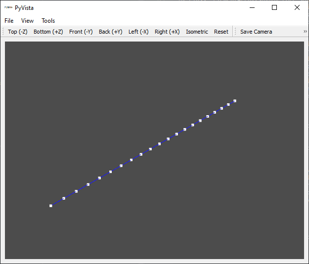
Geometry of the Beam
Systems in SDynPy
The System object is designed to
store the mass, stiffness, and damping matrices associated with a dynamic
system. These are stored in the mass, stiffness, and damping
attributes of the System object.
Typing system into the into the Python console will report the number of
the degrees of freedom in the system.
In [16]: system
Out[16]: System with 126 DoFs (126 internal DoFs)
We can plot the system matrices to see the element connectivity. Each matrix should have numbers of rows and columns equal to the reported number of internal degrees of freedom, which will be 126 for this
# Create the figure and axes
fig,ax = plt.subplots(1,3,sharex=True,sharey=True,num='System Matrices',
                      figsize=(12,3))
# Plot the matrices
mimg = ax[0].imshow(system.mass)
dimg = ax[1].imshow(system.damping)
simg = ax[2].imshow(system.stiffness)
# Add colorbar
plt.colorbar(mimg,ax=ax[0])
plt.colorbar(dimg,ax=ax[1])
plt.colorbar(simg,ax=ax[2])
# Label each plot
ax[0].set_title('Mass')
ax[1].set_title('Damping')
ax[2].set_title('Stiffness')
# Set to tight layout
fig.tight_layout()
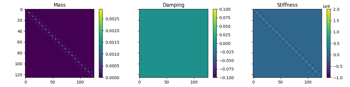
Mass, Stiffness, and Damping matrices for the system object.
Note that due to the system deriving from a finite element model, the damping is zero.
In addition to the mass, stiffness, and damping matrices, SDynPy
System objects also track
transformations between internal state degrees of freedom, as well as which
degrees of freedom are associated with rows and columns of the matrices.
For the current system object, the transformation, accessed using the
system.transformation attribute, is the identity matrix.
This is because the system matrices are already represented in physical
coordinates.
# Create the figure and axes
fig,ax = plt.subplots(1,1,sharex=True,sharey=True,num='System Transformation',
                      figsize=(4,3.5))
# Plot the matrices
timg = ax.imshow(system.transformation)
# Add colorbar
plt.colorbar(timg,ax=ax)
# Label each plot
ax.set_title('Transformation')
# Set to tight layout
fig.tight_layout()
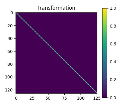
Transformation matrix for the system object.
The degrees of freedom corresponding to the rows and columns of the system
matrices can be accessed using the system.coordinate attribute. This
provides a CoordinateArray
object containing the degrees of freedom (node and local direction).
In [17]: system.coordinate
Out[17]:
coordinate_array(string_array=
array(['1X+', '1Y+', '1Z+', '1RX+', '1RY+', '1RZ+', '2X+', '2Y+', '2Z+',
       '2RX+', '2RY+', '2RZ+', '3X+', '3Y+', '3Z+', '3RX+', '3RY+',
       '3RZ+', '4X+', '4Y+', '4Z+', '4RX+', '4RY+', '4RZ+', '5X+', '5Y+',
       '5Z+', '5RX+', '5RY+', '5RZ+', '6X+', '6Y+', '6Z+', '6RX+', '6RY+',
       '6RZ+', '7X+', '7Y+', '7Z+', '7RX+', '7RY+', '7RZ+', '8X+', '8Y+',
       '8Z+', '8RX+', '8RY+', '8RZ+', '9X+', '9Y+', '9Z+', '9RX+', '9RY+',
       '9RZ+', '10X+', '10Y+', '10Z+', '10RX+', '10RY+', '10RZ+', '11X+',
       '11Y+', '11Z+', '11RX+', '11RY+', '11RZ+', '12X+', '12Y+', '12Z+',
       '12RX+', '12RY+', '12RZ+', '13X+', '13Y+', '13Z+', '13RX+',
       '13RY+', '13RZ+', '14X+', '14Y+', '14Z+', '14RX+', '14RY+',
       '14RZ+', '15X+', '15Y+', '15Z+', '15RX+', '15RY+', '15RZ+', '16X+',
       '16Y+', '16Z+', '16RX+', '16RY+', '16RZ+', '17X+', '17Y+', '17Z+',
       '17RX+', '17RY+', '17RZ+', '18X+', '18Y+', '18Z+', '18RX+',
       '18RY+', '18RZ+', '19X+', '19Y+', '19Z+', '19RX+', '19RY+',
       '19RZ+', '20X+', '20Y+', '20Z+', '20RX+', '20RY+', '20RZ+', '21X+',
       '21Y+', '21Z+', '21RX+', '21RY+', '21RZ+'], dtype='<U5'))
Coordinates
Here again is a good place to explore what makes up a
CoordinateArray
object. We can examine the data type of the
CoordinateArray
to see that it contains fields for a 64-bit unsigned integer as the node
field and an 8-bit signed integer for the direction field.
In [18]: system.coordinate.dtype
Out[18]: dtype([('node', '<u8'), ('direction', 'i1')])
CoordinateArray
objects store the direction as an integer with encoding:
Direction |
Integer Encoding |
|---|---|
X+ |
1 |
Y+ |
2 |
Z+ |
3 |
RX+ |
4 |
RY+ |
5 |
RZ+ |
6 |
X- |
-1 |
Y- |
-2 |
Z- |
-3 |
RX- |
-4 |
RY- |
-5 |
RZ- |
-6 |
None |
0 |
Note that the directions with R are rotations about the respective axis.
When we want to examine
CoordinateArray
objects, the integer directions are typically transformed into the more
readable direction strings shown in the first column of the above table. For
example, if we type a
CoordinateArray object
into the console, the representation of the
object displays the string array version of the coordinates, as shown above.
From the above, we can see that the
System we just created
contains a degree of freedom for each of the positive X, Y, Z translations and
each of the positive X, Y, Z rotations each node.
Many SDynPy objects allow indexing with a
CoordinateArray
object to automatically handle the bookkeeping aspect of selecting the right
data for each coordinate.
Plotting Coordinates
At this point, we would like to plot our coordinates on top of our geometry.
For this we use the
plot_coordinate
method of the Geometry object.
geometry.plot_coordinate(system.coordinate,arrow_scale=0.02)
Note that due to the density of the mesh, we had to make the arrow_scale
smaller than the default, otherwise the arrows would overlap.
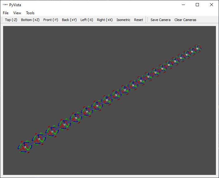
Coordinates defined on the beam.
If we zoom into the coordinate systems on the figure, we see more clearly that there are rotations and translations defined at each node.
Zoom of coordinates defined on the beam.
Computing Modes of the System
With mass, stiffness, and damping matrices, there are several types of
structural dynamics analyses that could be performed. One popular analysis
that is performed in structural dynamics is modal analysis. In this type of
analysis, we will compute the
Generalized Eigensolution
of the mass and stiffness matrices. While we could extract these matrices from
the System object and perform
the eigensolution using a linear algebra package such as that in SciPy, we can
instead use the System.eigensolution
method to compute the modes and handle all of the bookkeeping. This method
accepts arguments to determine which modes to compute. For example, we can
easily compute all modes below a certain frequency (say 4000 Hz).
shapes = system.eigensolution(maximum_frequency=4000)
This produces a ShapeArray
object, which is used by SDynPy to represent mode shapes and deflection shapes.
We can type the variable name shapes into the Python console to see more
information about the mode shapes.
In [19]: shapes
Out[19]:
   Index,  Frequency,    Damping,     # DoFs
    (0,),     0.0000,    0.0000%,        126
    (1,),     0.0000,    0.0000%,        126
    (2,),     0.0000,    0.0000%,        126
    (3,),     0.0153,    0.0000%,        126
    (4,),     0.0153,    0.0000%,        126
    (5,),     0.0153,    0.0000%,        126
    (6,),   648.5603,    0.0000%,        126
    (7,),  1297.1207,    0.0000%,        126
    (8,),  1787.8068,    0.0000%,        126
    (9,),  3504.9762,    0.0000%,        126
   (10,),  3575.6135,    0.0000%,        126
Here we see there were 11 modes below 4000 Hz. 6 of the modes are rigid body modes, with natural frequency of approximately 0 Hz. 5 of the modes are elastic modes. Each of the modes has 0% damping (due to the damping matrix being equal to the zero matrix), and each mode has 126 degrees of freedom.
Shapes
At this point, it is useful to explore briefly the
ShapeArray object in the
Python console. The data type of the object is:
In [20]: shapes.dtype
Out[20]: dtype([('frequency', '<f8'),
                ('damping', '<f8'),
                ('coordinate', [('node', '<u8'),
                                ('direction', 'i1')], (126,)),
                ('shape_matrix', '<f8', (126,)),
                ('modal_mass', '<f8'),
                ('comment1', '<U80'),
                ('comment2', '<U80'),
                ('comment3', '<U80'),
                ('comment4', '<U80'),
                ('comment5', '<U80')])
The data type of
ShapeArray objects can change
depending on what type of shape and how many degrees of freedom are in the
shape. frequency and damping fields are stored as 64-bit floating
point numbers with one value per entry in the
ShapeArray. modal_mass
is also stored in the present
ShapeArray, but if the shape
is complex, then the modal mass might also be complex. The shape_matrix
field holds the underlying shape data. It has one entry for every degree of
freedom in the shape, and is represented by a floating point number for
normal modes or a complex number for complex modes. Similarly, the
coordinate field identifies which degree of freedom belongs to which entry
in the shape_matrix field. The coordinate field stores data as
CoordinateArray
objects, and thus has the same data type as
CoordinateArray.
Finally, there are five fields available for comments, which store string data
up to 80 characters which can be used to store any data the user feels is
relevant to the analysis.
One thing to note is that the shape_matrix field, due to the dimension of
the field being appended at the end of the array, will be transposed from the
typical representation of a mode shape matrix (degrees of freedom as rows and
mode indices as columns). The shape_matrix field will instead have the
shape of the ShapeArray
object itself as its first dimensions, and then the size of the coordinate
field as its last dimension.
In [21]: shapes.shape
Out[21]: (11,)

In [22]: shapes.shape_matrix.shape
Out[22]: (11, 126)
To access the mode shape matrix in a more familiar format, users can instead
access the modeshape attribute of the
ShapeArray object. This will
be identical data to the shape_matrix field, except it will have the last
two dimensions of the array transposed. For a 1D array of shapes, this will
produce a modeshape matrix with degrees of freedom indices as the rows of the
matrix and mode indices as the columns of the matrix.
In [23]: shapes.modeshape.shape
Out[23]: (126, 11)
Plotting Shapes
While it may be useful to access the raw mode shape data in matrix form, the most
intutive view of the shapes is often obtained when the shapes are plotted on
the geometry. This is easily done in SDynPy by using the
plot_shape method of the
Geometry object, and passing
the ShapeArray object as the
argument.
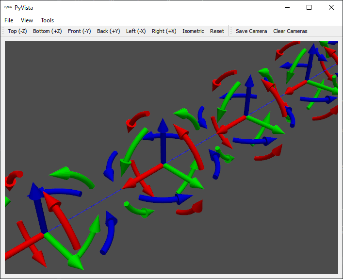
geometry.plot_shape(shapes)
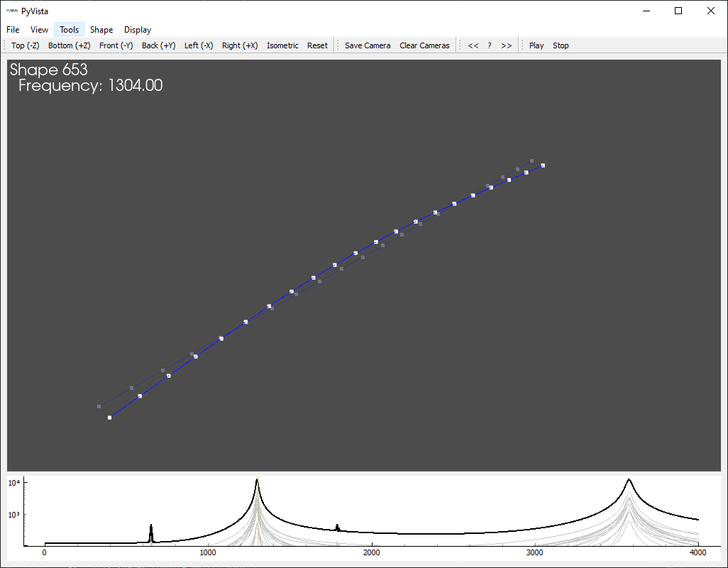
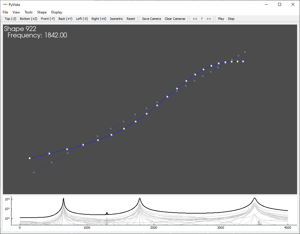
This will bring up the shape plotter window, shown below.
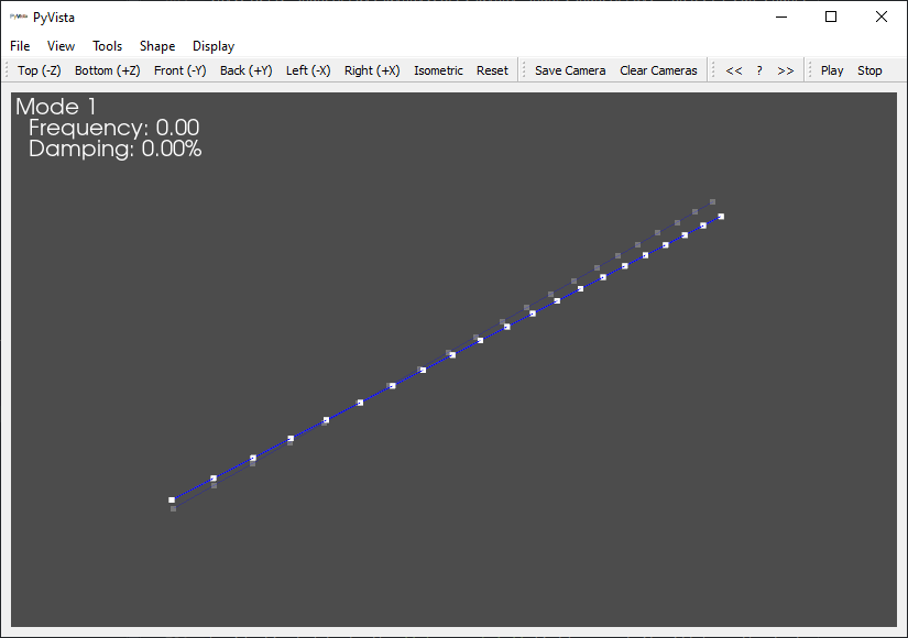
Shape Plotter window that appears when modes are plotted on the geometry.
The Shape Plotter window is an interactive, animated 3D plot that allows users to visualize the mode shapes of the system. We will briefly highlight some of the key features of this tool.
The File menu contains tools for saving images from the window. The
Take Screenshot action allows saving an image of the current window. The
Save Animation action will save an animated GIF of the shape from the
current view.
The View menu contains tools for adjusting the view of the window, as well
as plotting utility widgets. The Camera Toggle Parallel Projection
action will switch between perspective and parallel camera projections. A
small coordinate axis triad can be plotted by displaying the
Orientation Marker, and labelled axes can be plotted by selecting
Bounds Axes.
The Shape menu contains tools for adjusting how the shapes are presented.
The shape complexity can be adjusted, as well as the shape scaling and animation
speed. The text showing the mode number, frequency, damping, and any comments
can also be shown or hidden.
The toolbars in the widget offer features as well. The camera can be set to
several default views along the principal axes. Camera views can be saved and
recalled as well. The mode that is being shown can be changed by clicking the
<< and >> buttons. The animation can be started or stopped by pressing
the Play and Stop Buttons.
Mode shape of the beam animated on the geometry.
Assigning to SDynpy Array Fields and Array Views versus Copies
Often, one may wish to assign values to specific fields of the SDynPy objects.
For example, the first six modes of the structure should be rigid body modes;
however, the eigensolution has left three of the first six natural frequencies
with small positive values. Let’s set these values to zero. SDynPy arrays,
as well as the fields of the arrays, inherit all properties of NumPy’s
ndarray object, and can therefore be indexed identically. We can use this
indexing either to get specific portions of the array or to assign values to
certain portions of the array. For example, if we want to assign the first
six natural frequencies to zero, we can use the command:
shapes.frequency[:6] = 0
We can then check that the values are indeed set to zero.
In [24]: shapes
Out[24]:
   Index,  Frequency,    Damping,     # DoFs
    (0,),     0.0000,    0.0000%,        126
    (1,),     0.0000,    0.0000%,        126
    (2,),     0.0000,    0.0000%,        126
    (3,),     0.0000,    0.0000%,        126
    (4,),     0.0000,    0.0000%,        126
    (5,),     0.0000,    0.0000%,        126
    (6,),   648.5603,    0.0000%,        126
    (7,),  1297.1207,    0.0000%,        126
    (8,),  1787.8068,    0.0000%,        126
    (9,),  3504.9762,    0.0000%,        126
   (10,),  3575.6135,    0.0000%,        126
Note that when utilizing NumPy ndarray objects, one should always be aware
what type of object is returned from an indexing or slicing operation. NumPy
can either return a copy of the original array or a view into the original
array. A copy is a completely new array that contains equivalent data to the
original array, but has no connection back to it. Changing a value in a copy
of an array will not modify that same value in the original array. A view
is simply a window into the original array, meaning it shares the same memory
as the original array. Changing a value in a view of an array will also modify
the data in the original array. Views are useful in that they do not duplicate
memory, so when working with large arrays, using views is much more efficient
than using copies. However, if a user assumes that they are working with a
copy of an array but are actually working with a view of an array, there may
be unintended side-effects when the value of the original array is unintentionally
modified. For a full treatment of indexing in NumPy, users are directed to the
documentation on indexing
for NumPy ndarrays. The present documentation will simply show some examples
of when different types of indexing are used, and what the ramifications could
be if users are not careful.
Indexing using a Single Integer Index
The simplest indexing approach for NumPy objects is to index with a single
integer. This will generally return a view of the object. For example, we can
access the first shape in the
ShapeArray object with the
syntax
In [25]: first_shape = shapes[0]
If we then set the frequency of first_shape equal to some value, we will
see that our original shape matrix also has that value assigned as the first
frequency.
In [26]: first_shape.frequency = 10

In [27]: shapes
Out[27]:
   Index,  Frequency,    Damping,     # DoFs
    (0,),    10.0000,    0.0000%,        126
    (1,),     0.0000,    0.0000%,        126
    (2,),     0.0000,    0.0000%,        126
    (3,),     0.0000,    0.0000%,        126
    (4,),     0.0000,    0.0000%,        126
    (5,),     0.0000,    0.0000%,        126
    (6,),   648.5603,    0.0000%,        126
    (7,),  1297.1207,    0.0000%,        126
    (8,),  1787.8068,    0.0000%,        126
    (9,),  3504.9762,    0.0000%,        126
   (10,),  3575.6135,    0.0000%,        126
Here we see that we assigned a variable when we modified first_shape’s
frequency to 10, the first frequency of shapes also became 10, because they
point to the same position in memory.
Indexing using a Slice
A second common method of indexing an array is using a slice. Slices can be
defined with a start index, a stop index, and a step size. For example, a slice
0:10:2 would return indices from zero up to just before 10, and only return
every second index, which would be 0, 2, 4, 6, and 8.
For example:
In [29]: indexed_shapes = shapes[:6:2]

In [30]: indexed_shapes.frequency = 2

In [31]: shapes
Out[31]:
   Index,  Frequency,    Damping,     # DoFs
    (0,),     2.0000,    0.0000%,        126
    (1,),     0.0000,    0.0000%,        126
    (2,),     2.0000,    0.0000%,        126
    (3,),     0.0000,    0.0000%,        126
    (4,),     2.0000,    0.0000%,        126
    (5,),     0.0000,    0.0000%,        126
    (6,),   648.5603,    0.0000%,        126
    (7,),  1297.1207,    0.0000%,        126
    (8,),  1787.8068,    0.0000%,        126
    (9,),  3504.9762,    0.0000%,        126
   (10,),  3575.6135,    0.0000%,        126
We can see that the 0, 2, and 4 indices were set to have frequencies of 2, which corresponds to the original slice.
Note we could also do the indexing directly on the frequency field.
For example:
In [32]: indexed_frequencies = shapes.frequency[:6:2]

In [33]: indexed_frequencies[:] = 3

In [34]: shapes
Out[34]:
   Index,  Frequency,    Damping,     # DoFs
    (0,),     3.0000,    0.0000%,        126
    (1,),     0.0000,    0.0000%,        126
    (2,),     3.0000,    0.0000%,        126
    (3,),     0.0000,    0.0000%,        126
    (4,),     3.0000,    0.0000%,        126
    (5,),     0.0000,    0.0000%,        126
    (6,),   648.5603,    0.0000%,        126
    (7,),  1297.1207,    0.0000%,        126
    (8,),  1787.8068,    0.0000%,        126
    (9,),  3504.9762,    0.0000%,        126
   (10,),  3575.6135,    0.0000%,        126
Note the syntax indexed_frequencies[:] = 3. Had we simply typed
indexed_frequencies = 3, this would have not overwritten the original
frequencies as this latter syntax is simply a redefinition of the variable
indexed_frequencies to a different value rather than a reassignment of the
values in indexed_frequencies to a different value. The former syntax
reassigns values at the indexed_frequencies memory location, and the latter
assigns indexed_frequencies to a different memory location, which breaks
the connection to the original memory location, so indexed_frequencies is
no longer a view into shapes. For example:
In [35]: indexed_frequencies = 6

In [36]: shapes
Out[36]:
   Index,  Frequency,    Damping,     # DoFs
    (0,),     3.0000,    0.0000%,        126
    (1,),     0.0000,    0.0000%,        126
    (2,),     3.0000,    0.0000%,        126
    (3,),     0.0000,    0.0000%,        126
    (4,),     3.0000,    0.0000%,        126
    (5,),     0.0000,    0.0000%,        126
    (6,),   648.5603,    0.0000%,        126
    (7,),  1297.1207,    0.0000%,        126
    (8,),  1787.8068,    0.0000%,        126
    (9,),  3504.9762,    0.0000%,        126
   (10,),  3575.6135,    0.0000%,        126
In the previous example the values of the 0, 2, and 4 frequency indices were not modified from three to six.
Indexing with Logical Arrays
NumPy ndarrays can also be indexed with logical (or boolean) arrays. These
are arrays full of True and False values. These are often returned due
to comparison operations. For example, if we want all of the frequencies less
than ten hertz, we can perform the operation:
In [37]: logical_array = shapes.frequency < 10

In [38]: logical_array
Out[38]:
array([ True,  True,  True,  True,  True,  True, False, False, False,
       False, False])
This last set of commands has produced a logical array where the first six
indices are True and the last five are False. If we index the shapes
object with this, we will return only the shapes where the logical array is
True.
In [39]: rigid_shapes = shapes[logical_array]

In [40]: rigid_shapes
Out[40]:
   Index,  Frequency,    Damping,     # DoFs
    (0,),     3.0000,    0.0000%,        126
    (1,),     0.0000,    0.0000%,        126
    (2,),     3.0000,    0.0000%,        126
    (3,),     0.0000,    0.0000%,        126
    (4,),     3.0000,    0.0000%,        126
    (5,),     0.0000,    0.0000%,        126
However, unlike the last indexing types, this type of indexing will generally
return a copy of the array, rather than a view into the array. For example,
if we redefine values of the frequency field in rigid_shapes, it will
not update the frequency in the original shapes variable.
In [41]: rigid_shapes.frequency = 0

In [42]: rigid_shapes
Out[42]:
   Index,  Frequency,    Damping,     # DoFs
    (0,),     0.0000,    0.0000%,        126
    (1,),     0.0000,    0.0000%,        126
    (2,),     0.0000,    0.0000%,        126
    (3,),     0.0000,    0.0000%,        126
    (4,),     0.0000,    0.0000%,        126
    (5,),     0.0000,    0.0000%,        126

In [43]: shapes
Out[43]:
   Index,  Frequency,    Damping,     # DoFs
    (0,),     3.0000,    0.0000%,        126
    (1,),     0.0000,    0.0000%,        126
    (2,),     3.0000,    0.0000%,        126
    (3,),     0.0000,    0.0000%,        126
    (4,),     3.0000,    0.0000%,        126
    (5,),     0.0000,    0.0000%,        126
    (6,),   648.5603,    0.0000%,        126
    (7,),  1297.1207,    0.0000%,        126
    (8,),  1787.8068,    0.0000%,        126
    (9,),  3504.9762,    0.0000%,        126
   (10,),  3575.6135,    0.0000%,        126
Here we see that there is no memory link between rigid_shapes and shapes
because they have different values of their frequency field. Note that if
we wish to perform assignments using logical indexing, we need to make sure that
the indexing is performed as the last operation. For example, consider the
following code.
In [44]: shapes[logical_array].frequency = 0

In [45]: shapes
Out[45]:
   Index,  Frequency,    Damping,     # DoFs
    (0,),     3.0000,    0.0000%,        126
    (1,),     0.0000,    0.0000%,        126
    (2,),     3.0000,    0.0000%,        126
    (3,),     0.0000,    0.0000%,        126
    (4,),     3.0000,    0.0000%,        126
    (5,),     0.0000,    0.0000%,        126
    (6,),   648.5603,    0.0000%,        126
    (7,),  1297.1207,    0.0000%,        126
    (8,),  1787.8068,    0.0000%,        126
    (9,),  3504.9762,    0.0000%,        126
   (10,),  3575.6135,    0.0000%,        126
Looking at the first command naively, it would seem that we would take the
shapes specified by logical_array (i.e. the first six modes) and assign their
frequencies to 0. However, if we look at the contents of shapes immediately
afterwards, we can see that no such assignment has taken place. Instead, the
first six modes have their original values of alternating three and zero.
If we think a bit harder and remember that we make a copy of the array when we
index with a logical array, we will realize that we have created a copy of the
first six modes of the shapes array, and assigned the frequencies of that
copy to zero. However, since that copy was never assigned to any variable, it
is immediately discarded by the Python interpreter as unused. The original
shapes array remains unmodified. To achieve the desired result, we should
instead make sure the indexing occurs last.
In [46]: shapes.frequency[logical_array] = 0

In [47]: shapes
Out[47]:
   Index,  Frequency,    Damping,     # DoFs
    (0,),     0.0000,    0.0000%,        126
    (1,),     0.0000,    0.0000%,        126
    (2,),     0.0000,    0.0000%,        126
    (3,),     0.0000,    0.0000%,        126
    (4,),     0.0000,    0.0000%,        126
    (5,),     0.0000,    0.0000%,        126
    (6,),   648.5603,    0.0000%,        126
    (7,),  1297.1207,    0.0000%,        126
    (8,),  1787.8068,    0.0000%,        126
    (9,),  3504.9762,    0.0000%,        126
   (10,),  3575.6135,    0.0000%,        126
In this latter case, we have accessed the frequency field of the original
shapes array, rather than a copy of the frequency field, therefore when
we assign to those values, the original shapes array is modified.
Indexing with Integer Arrays
The final indexing approach discussed here is indexing with integer arrays. This is useful when specific indices are desired, but one does not want to set up the entire logical array. For example, to get the first six modes, we could construct an integer array:
In [48]: integer_array = [0,1,2,3,4,5]

In [49]: rigid_shapes = shapes[integer_array]

In [50]: rigid_shapes
Out[50]:
   Index,  Frequency,    Damping,     # DoFs
    (0,),     0.0000,    0.0000%,        126
    (1,),     0.0000,    0.0000%,        126
    (2,),     0.0000,    0.0000%,        126
    (3,),     0.0000,    0.0000%,        126
    (4,),     0.0000,    0.0000%,        126
    (5,),     0.0000,    0.0000%,        126
We can see that we were able to access the first six modes of shapes this
way.
In [51]: rigid_shapes.frequency = 10

In [52]: shapes
Out[52]:
   Index,  Frequency,    Damping,     # DoFs
    (0,),     0.0000,    0.0000%,        126
    (1,),     0.0000,    0.0000%,        126
    (2,),     0.0000,    0.0000%,        126
    (3,),     0.0000,    0.0000%,        126
    (4,),     0.0000,    0.0000%,        126
    (5,),     0.0000,    0.0000%,        126
    (6,),   648.5603,    0.0000%,        126
    (7,),  1297.1207,    0.0000%,        126
    (8,),  1787.8068,    0.0000%,        126
    (9,),  3504.9762,    0.0000%,        126
   (10,),  3575.6135,    0.0000%,        126
We can see that the changes to rigid_shapes were not propogated back to
shapes, because it is only a copy of the original array.
As a general rule of thumb, indexing using a single integer or slice produces a view into the original array, but indexing with a logical or index array produces a copy. If the reader still does not understand these concepts, they are encouraged to read and understand the NumPy documentation on indexing, otherwise misapplying these nuanced concepts can introduce bugs into analyses performed using SDynPy.
Computing a Modal System
Given that our ShapeArray object
came from a beam finite element model without any damping defined, it might be
useful to assign damping to the shapes to more realistically simulate a real
beam. We will assign a small amount of damping to all modes.
shapes.damping = 0.005
Now, if we investigate the shapes variable in the console, we will see
that the damping is no longer zero.
In [53]: shapes
Out[53]:
   Index,  Frequency,    Damping,     # DoFs
    (0,),     0.0000,    0.5000%,        126
    (1,),     0.0000,    0.5000%,        126
    (2,),     0.0000,    0.5000%,        126
    (3,),     0.0000,    0.5000%,        126
    (4,),     0.0000,    0.5000%,        126
    (5,),     0.0000,    0.5000%,        126
    (6,),   648.5603,    0.5000%,        126
    (7,),  1297.1207,    0.5000%,        126
    (8,),  1787.8068,    0.5000%,        126
    (9,),  3504.9762,    0.5000%,        126
   (10,),  3575.6135,    0.5000%,        126
If we wanted to perform simulations with this new model that has damping
incorporated, we can easily transform the
ShapeArray object into a
System object by using the
system method of the
ShapeArray class.
modal_system = shapes.system()
This will construct a System
object, but unlike our original system variable, this modal_system will
be a reduced system. Instead of the internal system states being equivalent
to physical degrees of freedom, the internal system states are now modal
degrees of freedom.
If we type the modal_system variable into the console, we see that while it
still has 126 degrees of freedom, it only contains 11 internal degrees of
freedom.
In [53]: modal_system
Out[53]: System with 126 DoFs (11 internal DoFs)
We can plot the system matrices.
# Plot the modal system matrices
fig,ax = plt.subplots(1,4,num='Modal System Matrices',figsize=(12,3))
# Transformation
timg = ax[0].imshow(modal_system.transformation)
ax[0].set_title('Transformation')
ax[0].set_ylabel('Physical DoF')
ax[0].set_xlabel('Modal DoF')
plt.colorbar(timg,ax=ax[0])
# Mass
mimg = ax[1].imshow(modal_system.mass)
ax[1].set_title('Mass')
ax[1].set_ylabel('Modal DoF')
ax[1].set_xlabel('Modal DoF')
plt.colorbar(mimg,ax=ax[1])
# Damping
dimg = ax[2].imshow(modal_system.damping)
ax[2].set_title('Damping')
ax[2].set_ylabel('Modal DoF')
ax[2].set_xlabel('Modal DoF')
plt.colorbar(dimg,ax=ax[2])
# Stiffness
simg = ax[3].imshow(modal_system.stiffness)
ax[3].set_title('Stiffness')
ax[3].set_ylabel('Modal DoF')
ax[3].set_xlabel('Modal DoF')
plt.colorbar(simg,ax=ax[3])
fig.tight_layout()
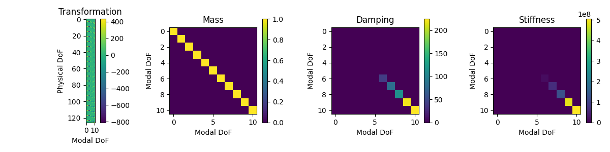
Transformation, Mass, Damping and System matrices for the modal_system
object.
We can see that the mass, stiffness, and
damping matrices of modal_system are now the modal mass, modal stiffness,
and modal damping matrices. SDynPy also tracks the transformation between internal
degrees of freedom and physical degrees of freedom, which in this case is the
mode shape matrix \(\mathbf{\Phi}\), which transforms modal degrees of freedom \(\mathbf{q}\)
to physical degrees of freedom \(\mathbf{x}\) by the well-known modal
transformation
We can see that the coordinates of the original system and modal_system
are identical, meaning the same physical degrees of freedom exist in each.
In [54]: np.all(system.coordinate == modal_system.coordinate)
Out[54]: True
Because SDynPy tracks the transformation between internal and physical degrees
of freedom and applies it when necessary, the reduced modal_system can be
utilized identically to the original system consisting of physical degrees
of freedom. For example, we can compute the eigensolution of modal_system
and find that it produces the exact same modes as the original shapes. The
transformation is automatically applied to the mode shape matrix to produce
shapes at the physical degrees of freedom.
In [55]: modal_system.eigensolution()
Out[55]:
   Index,  Frequency,    Damping,     # DoFs
    (0,),     0.0000,    0.0000%,        126
    (1,),     0.0000,    0.0000%,        126
    (2,),     0.0000,    0.0000%,        126
    (3,),     0.0000,    0.0000%,        126
    (4,),     0.0000,    0.0000%,        126
    (5,),     0.0000,    0.0000%,        126
    (6,),   648.5603,    0.5000%,        126
    (7,),  1297.1207,    0.5000%,        126
    (8,),  1787.8068,    0.5000%,        126
    (9,),  3504.9762,    0.5000%,        126
   (10,),  3575.6135,    0.5000%,        126
The modal system is useful because it can give approximately the same results as the physical system (at least over the bandwidth of interest) with significantly less computational cost. Rather than performing computations on a coupled, 126-degree-of-freedom system, we can instead perform computations on an uncoupled, 11-degree-of-freedom system, and then apply a simple transformation to convert the results back to physical degrees of freedom.
Data in SDynPy
Data in SDynPy is stored as subclasses of the
NDDataArray object, which
represents all types of data in SDynPy (time histories, frequency response
functions, power spectral density arrays, etc.). Functionality for specific
data types are stored in their respective subclasses. For example, time history
signals are stored in
TimeHistoryArray objects
and frequency response functions are stored in
TransferFunctionArray
objects.
In general, to create a
NDDataArray object, users will
utilize the
data_array function. This
function accepts a type specifier defined by the
FunctionTypes enumeration.
It will also accept the abscissa (independent variable, e.g., frequency or time),
the ordinate (dependent variable, e.g., acceleration or force), the coordinate
(degree of freedom information for the signal), as well as up to five comments.
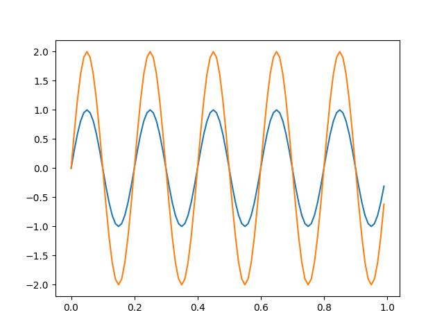
For example, we can construct a set of sine waves with different amplitudes
times = np.arange(100)/100
amplitudes = np.array([1,2])
signal = amplitudes[:,np.newaxis]*np.sin(2*np.pi*5*times)
coordinates = sdpy.coordinate_array(
    string_array=['101X+','101Y-'])[:,np.newaxis]

time_history = sdpy.data_array(
    data_type = sdpy.data.FunctionTypes.TIME_RESPONSE,
    abscissa = times,
    ordinate = signal,
    coordinate = coordinates)
There are numerous function types defined in SDynPy. Referencing the
sdpy.data module will show the different
subclasses available.
Let’s take this time to explore of the
NDDataArray class before moving
on. First, let’s examine the fields available by looking at the object’s
dtype.
In [56]: time_history.dtype
Out[56]: dtype([('abscissa', '<f8', (100,)),
                ('ordinate', '<f8', (100,)),
                ('comment1', '<U80'),
                ('comment2', '<U80'),
                ('comment3', '<U80'),
                ('comment4', '<U80'),
                ('comment5', '<U80'),
                ('coordinate', [('node', '<u8'),
                                ('direction', 'i1')], (1,))])
The abscissa field consists of the independent variable, which in the case
of this time history, is the time value at each step. Different function types
will have different abscissa data types. For example, a spectral quantity may
have frequency lines as its abscissa. The ordinate field consists of the
dependant variable. For a time history, this is a real quantity, but for a
frequency-domain function such as a frequency response function, this may be a
complex value. Both abscissa and ordinate have a shape of (100,), which
is the length of the time signal. Like the
ShapeArray,
there are five fields available for comments, which store string data
up to 80 characters which can be used to store any data the user feels is
relevant to the analysis. Finally, the coordinate field stores degree of
freedom data as
CoordinateArray
objects, and thus has the same data type as
CoordinateArray.
Different function types will have different shaped coordinate fields.
For example, a time history only has one degree of freedom associated with each
signal, so its shape is (1,). Note, however that this makes the coordinate
field for the entire array (2,1), which is why the new axis needed to be
added to the coordinates coordinates variable in the previous code block.
In [57]: time_history.shape
Out[57]: (2,)

In [58]: time_history.coordinate.shape
Out[58]: (2, 1)
Other types of functions may have differently-shaped coordinate fields.
For example, a frequency response function will generally have a response
coordinate and a reference coordinate for each entry in the matrix, so it will
have a coordinate field of shape (2,).
There are many ways to visualize data in SDynPy, but the simplest is generally
to call the
plot method of the
NDDataArray object.
time_history.plot()
This will produce a plot window with the signals displayed in it. This is more useful for smaller datasets. The plots produced by this method can get quite busy if many signals are plotted.
Integrating Equations of Motion to Produce Time Data
While NDDataArray objects can
be created manually, many functions and methods in SDynPy will return various
data. One common operation is to integrate the equations of motion of a system
to create a simulated time response to an imposed excitation or an imposed
initial condition. The
time_integrate
method of the System class can be
used to integrate the dynamic system to produce time responses. We will
demonstrate this analysis in this section.
Generating an Excitation Signal
When setting up the time integration, we must consider the excitation that will
be applied to the System, as well
as the initial conditions. For this case, we will consider the system starting
at rest. We will excite the structure with a pair of perpendicular random
vibration signals at the beam tip. We can easily create these signals using
SDynPy’s sdpy.generator
sub-module. This contains functions to produce common signals used in
structural dynamics such as
sine,
chirp,
pseudorandom,
random,
burst_random,
and pulse.
We will look at the random
function to generate the input signals for this analysis. We will set up some
initial signal processing parameters prior to generating the signal.
# Set up sampling parameters
signal_bandwidth = 4000 # Hz
sample_rate = signal_bandwidth*2
dt = 1/sample_rate
samples_per_frame = 2000
num_frames = 30
total_samples = samples_per_frame*num_frames
rms_level = 1.0
num_signals = 2

# Generate the signals
signals = sdpy.generator.random((num_signals,),total_samples,rms_level,dt)

# Plot the signals
fig,ax = plt.subplots(num_signals,1,num='Random Signals',
                      sharex=True,sharey=True)
ax[0].plot(np.arange(total_samples)*dt,signals[0],linewidth=0.5)
ax[0].set_ylabel('Signal 1 (N)')
ax[1].plot(np.arange(total_samples)*dt,signals[1],linewidth=0.5)
ax[1].set_ylabel('Signal 2 (N)')
ax[1].set_xlabel('Time (s)')
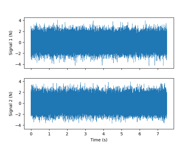
Random signal used to excite the structure
Performing the Time Integration
We can then apply the signal to the structure using the
time_integrate
method of the System class.
We need to chose which degrees of freedom to plot on the structure. Recall
we can plot degrees of freedom using the
plot_coordinate
method of the Geometry object.
By not specifying a set of coordinates to plot, it will simply plot all
translational coordinates. Additionally, we can pass the optional keyword
argument label_dofs = True to tell the plotter to label the degrees of
freedom in the plot.
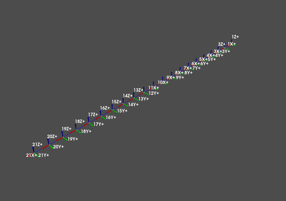
geometry.plot_coordinate(label_dofs=True,arrow_scale=0.02)
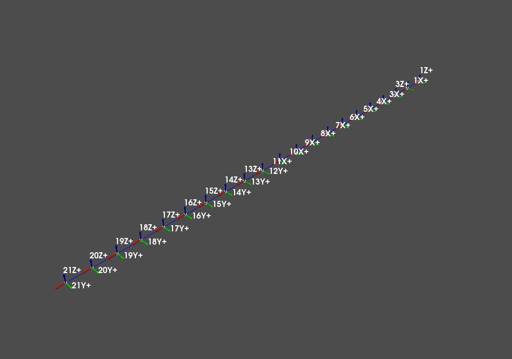
Beam geometry with coordinate labels plotted
We will place the excitation forces at the tip of the beam in the two transverse
directions. This corresponds to degrees of freedom 21Y+ and 21Z+.
We can define a new coordinate array using the
sdpy.coordinate_array
function. This function can define new
CoordinateArray
objects in multiple ways. In this case, we will provide it the string_array
keyword argument, and pass the coordinates that we desire in as strings.
Alternatively, they could also be passed in as separate nodes and directions,
which is useful for longer coordinate arrays.
excitation_dofs = sdpy.coordinate_array(
    string_array = ['21Y+','21Z+'])

geometry.plot_coordinate(excitation_dofs,label_dofs=True,arrow_scale=0.05)
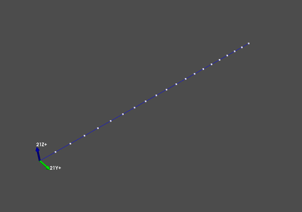
Excitation degrees of freedom plotted on the beam geometry
We might also specify the degrees of freedom at which we would like responses.
One could argue that it is quite difficult to measure rotations of a structure,
so we could construct our simulation such that it only returns the translational
degrees of freedom. We can easily get a list of all translational degrees of
freedom using the
sdpy.coordinate.from_nodelist
function, which accepts a list of nodes and returns translational degrees of
freedom (by default, though can be modified) at each node in the list. We can
generate this list of node identification numbers from our geometry object.
response_dofs = sdpy.coordinate.from_nodelist(geometry.node.id)
geometry.plot_coordinate(response_dofs,label_dofs=True,arrow_scale=0.025)
Response degrees of freedom plotted on the beam geometry
We can then integrate equations of motion for the system using the
time_integrate
method of the System.
responses,forces = modal_system.time_integrate(
    signals, dt, responses = response_dofs, references=excitation_dofs,
    displacement_derivative = 2,
    integration_oversample = 10)
In addition to variables previously defined, we have also defined keyword
arguments displacement_derivative = 2 and integration_oversample = 10.
The displacement_derivative keyword specifies what data type to return.
Specifying a two for this value will return an acceleration quantity, which is
the second derivative of displacement. Specifying zero or one for this value
will result in displacement or velocity being returned, respectively.
The integration_oversample keyword determines the degree of oversampling
that occurs in the integration. The defined forces used a sample rate of
8000 Hz, so an oversample value of 10 will result in an integration time step
of 80000 steps per second of integration time. One must be wary of using this
keyword argument, as it relies on zero-padding the Fourier Transform of the
signal, which is not an appropriate approach to oversample certain functions.
For example, if the excitation is a ramp, this zero-padding will produce
strange end effects. If such a signal is used as the excitation, it is
recommended to simply generate the signal such that it is already oversampled,
and not use the integration_oversample argument of this function.
Note also that the
scipy.signal.lsim
function is used to perform the integration, so a factor of 10x is generally
sufficient for integration accuracy due to the linear system assumption.
Let’s investigate the output of the
time_integrate
method. Two outputs were produced, responses and forces. These are the
responses to the input signal, as well as the input signal itself, both
transformed into SDynPy
TimeHistoryArray objects.
In [59]: responses
Out[59]: TimeHistoryArray with shape 63 and 60000 elements per function

In [60]: forces
Out[60]: TimeHistoryArray with shape 2 and 60000 elements per function
Here we see that there are 63 response signals, and 2 force signals.
Here is an example where using the basic
plot method of the
TimeHistoryArray object
may be unsatisfactory, as too many lines will be plotted on the figure. Instead
we will use the interactive 2D plotter
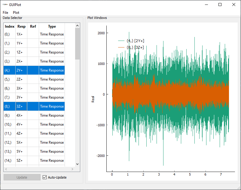
GUIPlot, which will allow us to
interactively chose which signals to show.
In [61]: sdpy.GUIPlot(responses)
Out[61]: <sdynpy.core.sdynpy_data.GUIPlot at 0xXXXXXXXXXXX>
Another approach to visualizing the response of the system is to plot it.
Plotting displacements is perhaps more meaningful than plotting accelerations,
which we have computed here. Nonetheless, it is valuable to show how this
can be done in SDynPy. The
plot_transient
method of the Geometry object
can be used to show the time responses as displacements on the geometry.
In [62]: geometry.plot_transient(responses,displacement_scale=0.003)
Out[62]: <sdynpy.core.sdynpy_geometry.TransientPlotter at 0xXXXXXXXXXXX>
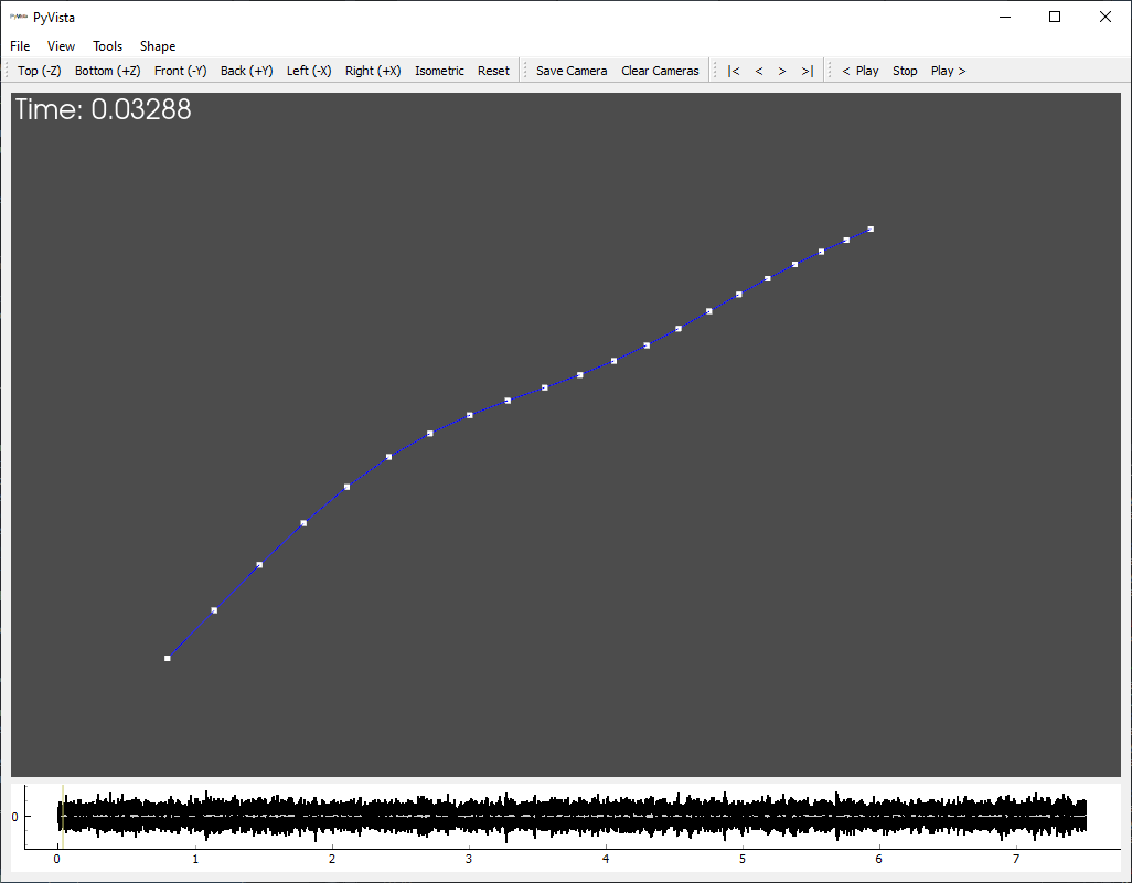
TransientPlotter
showing the acceleration shape at each time step in the analysis
The transient plotter is similar to the mode shape plotter shown previously,
except instead of animating a single shape vibrating back and forth, it animates
a series of shapes one after another. The user can adjust the current timestep
using the |<, <, >, or >| buttons, or by sliding the cursor
across the time history representation at the bottom of the window.
The animation can be started by clicking one of the < Play or Play >
buttons, which will plan the animation in reverse or forward, respectively. The
animation can be stopped by clicking the Stop button. The Shape menu
has options for scaling the displacement level and animation speed, as well as
setting the animation to loop.
Computing Frequency Response Functions
SDynPy offers several approaches to compute frequency response functions.
These can be computed directly from a
System object using its
frequency_response method,
in which the dynamic stiffness matrix will be inverted and transformations
applied. Frequency response functions can also be computed from
ShapeArray objects using its
compute_frf method.
Finally, frequency response functions can be computed from
TimeHistoryArray using
the
sdpy.TransferFunctionArray.from_time_data
function, or alternatively the
SignalProcessingGUI.
Code-based Frequency Response Function Computations
Let’s set up some initial parameters to use to compute frequency response functions.
df = 1/(dt*samples_per_frame)
frequency_lines = df*(np.arange(samples_per_frame)+1)
Then we can compute the frequency response functions with the approaches described above. First we will consider the code-based approaches.
# From the original undamped system
frfs_system = system.frequency_response(frequency_lines,
                                        response_dofs,
                                        excitation_dofs,
                                        displacement_derivative=2)
# From the reduced system with damping added
frfs_modal_system = modal_system.frequency_response(
    frequency_lines,
    response_dofs,
    excitation_dofs,
    displacement_derivative=2)
# From the eigensolution
frfs_shapes = shapes.compute_frf(frequency_lines,
                                 response_dofs,
                                 excitation_dofs,
                                 displacement_derivative=2)
# From time data
frfs_time = sdpy.TransferFunctionArray.from_time_data(
    forces, responses, samples_per_frame,
    overlap = 0.5, window = 'hann')
Before we go too much further, let’s explore the
sdpy.TransferFunctionArray
object returned by these analyses. First, by typing the variable name into
the console, we can see the shape of the
sdpy.TransferFunctionArray
as well as how many elements (frequency lines) are in each function.
In [63]: frfs_system
Out[63]: TransferFunctionArray with shape 63 x 2 and 1000 elements per function
We can also examine the dtype of the
sdpy.TransferFunctionArray,
in particular comparing it to that of the
TimeHistoryArray
In [64]: responses.dtype
Out[64]: dtype([('abscissa', '<f8', (60000,)),
                ('ordinate', '<f8', (60000,)),
                ('comment1', '<U80'),
                ('comment2', '<U80'),
                ('comment3', '<U80'),
                ('comment4', '<U80'),
                ('comment5', '<U80'),
                ('coordinate', [('node', '<u8'),
                                ('direction', 'i1')], (1,))])

In [65]: frfs_system.dtype
Out[65]: dtype([('abscissa', '<f8', (1000,)),
                ('ordinate', '<c16', (1000,)),
                ('comment1', '<U80'),
                ('comment2', '<U80'),
                ('comment3', '<U80'),
                ('comment4', '<U80'),
                ('comment5', '<U80'),
                ('coordinate', [('node', '<u8'),
                                ('direction', 'i1')], (2,))])
Because both the
sdpy.TransferFunctionArray
frfs_system and the
TimeHistoryArray responses
are subclasses of the base NDDataArray
class, which represents all data in SDynPy, they will have the same fields.
However, the shapes and data types of the fields are different. We see that the
ordinate field of the
TimeHistoryArray object
is a floating point number f8, whereas the ordinate field of the
sdpy.TransferFunctionArray
object is a complex number c16, because in general, frequency response
functions are complex. Additionally, we see that the the coordinate field
now no longer has shape (1,), but now has shape (2,). This is because
there are two degrees of freedom associated with each entry in the frequency
response function matrix, a response coordinate and a reference coordinate.
In each of the frequency response functions we have computed, there are 63 responses and 2 forces, meaning a total of 126 frequency response functions have been generated. Rather than comparing all of these functions, we will just compare the drive point frequency response functions. This can be easily selected by identifying the functions where the response coordinate is equal to the reference coordinate (allowing for a difference in sign to occur between the two).
drive_frfs_system = frfs_system[
    np.where(
        abs(frfs_system.response_coordinate)
        ==
        abs(frfs_system.reference_coordinate))]

drive_frfs_modal_system = frfs_modal_system[
    np.where(
        abs(frfs_modal_system.response_coordinate)
        ==
        abs(frfs_modal_system.reference_coordinate))]

drive_frfs_shapes = frfs_shapes[
    np.where(
        abs(frfs_shapes.response_coordinate)
        ==
        abs(frfs_shapes.reference_coordinate))]

drive_frfs_time = frfs_time[
    np.where(
        abs(frfs_time.response_coordinate)
        ==
        abs(frfs_time.reference_coordinate))]
We can then plot the drive point frequency response functions on the same plots to compare them.
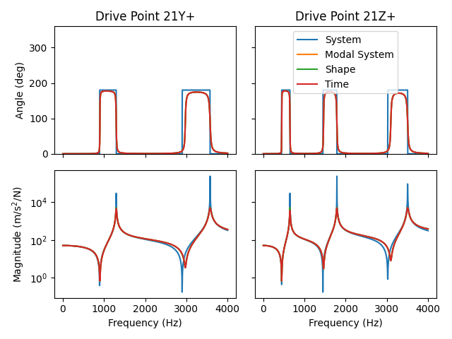
Frequency response functions computed from different approaches.
It may aid understanding to zoom in on a specific peak of the frequency response function to understand the subtle differences between the approaches.
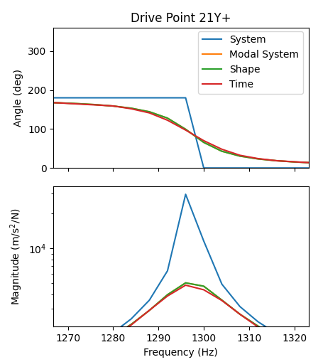
Zoom of frequency response functions computed from different approaches.
The most obvious difference between the four plots is in the System plot.
This original system, derived from a finite element model, had no damping
associated with it. Therefore the peak is very sharp (indeed, infinitely sharp
if we had plotted with infinite frequency resolution) compared to the other
three where we had added 0.5% modal damping. The Modal System and Shape
derived frequency response functions are nominally identical due to them being
constructed from nominally identical data. Finally, the Time curve is slightly
more blunt than the Shape or Modal System curves due to the artificial
damping added to the system from the Hann window applied during the frequency
response function computation.
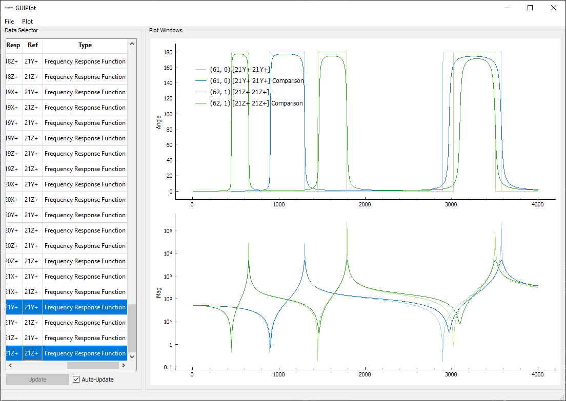
If users would like to compare all frequency response functions rather than just
the drive points, the GUIPlot is
again helpful. Two data sets can be passed simultaneously into the class
to allow for comparisons of large datasets to be performed interactively.
SDynPy by default plots frequency response functions as log magnitude and phase.
However, the complex plotting and logarithmic scaling of the axes can be modified
in the Plot menu.
Mode Indicator Functions
Another way to perform data reduction from a large number of frequency response functions to an overall view of the system is to compute mode indicator functions. Most popular are the Complex Mode Indicator Function (CMIF), the Normal Mode Indicator Function (NMIF), and the Multi-Mode Indicator Function (MMIF). One may also hear of the QMIF, which is a variant of the CMIF that is computed using only the imaginary part of the frequency response function (or real part when considering velocity/force frequency response functions).
SDynPy can compute the mode indicator functions using the
compute_cmif,
compute_nmif,
and
compute_mmif
methods of the
sdpy.TransferFunctionArray
object. See their respective documentation for additional arguments that
can be passed to these functions.
# CMIF
ax = frfs_shapes.compute_cmif().plot()
ax.set_xlabel('Frequency (Hz)')
ax.set_ylabel('CMIF')
# NMIF
ax = frfs_shapes.compute_nmif().plot()
ax.set_xlabel('Frequency (Hz)')
ax.set_ylabel('NMIF')
# MMIF
ax = frfs_shapes.compute_mmif().plot()
ax.set_xlabel('Frequency (Hz)')
ax.set_ylabel('MMIF')
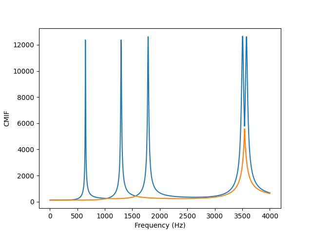
Complex mode indicator function for the beam frequency response functions
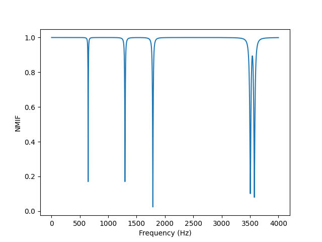
Normal mode indicator function for the beam frequency response functions
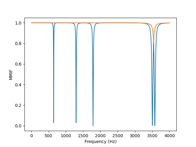
Multi-mode indicator function for the beam frequency response functions
Graphical Frequency Response Function Computation
While code-based frequency response function computations are nice in that they
can be automated very easily, some users may prefer a more graphical approach.
The SignalProcessingGUI
provides a way to do this. We pass it all of our time histories (references and
responses) and then a window appears which provides various signal processing
parameters that can be selected.
# Concatenate all time signals into one array
all_time_data = np.concatenate((forces,responses))
# Pass the entire set of time histories into the SignalProcessingGUI
spgui = sdpy.SignalProcessingGUI(all_time_data)
# Assign the geometry to the GUI so we don't have to load it from disk
spgui.geometry = geometry
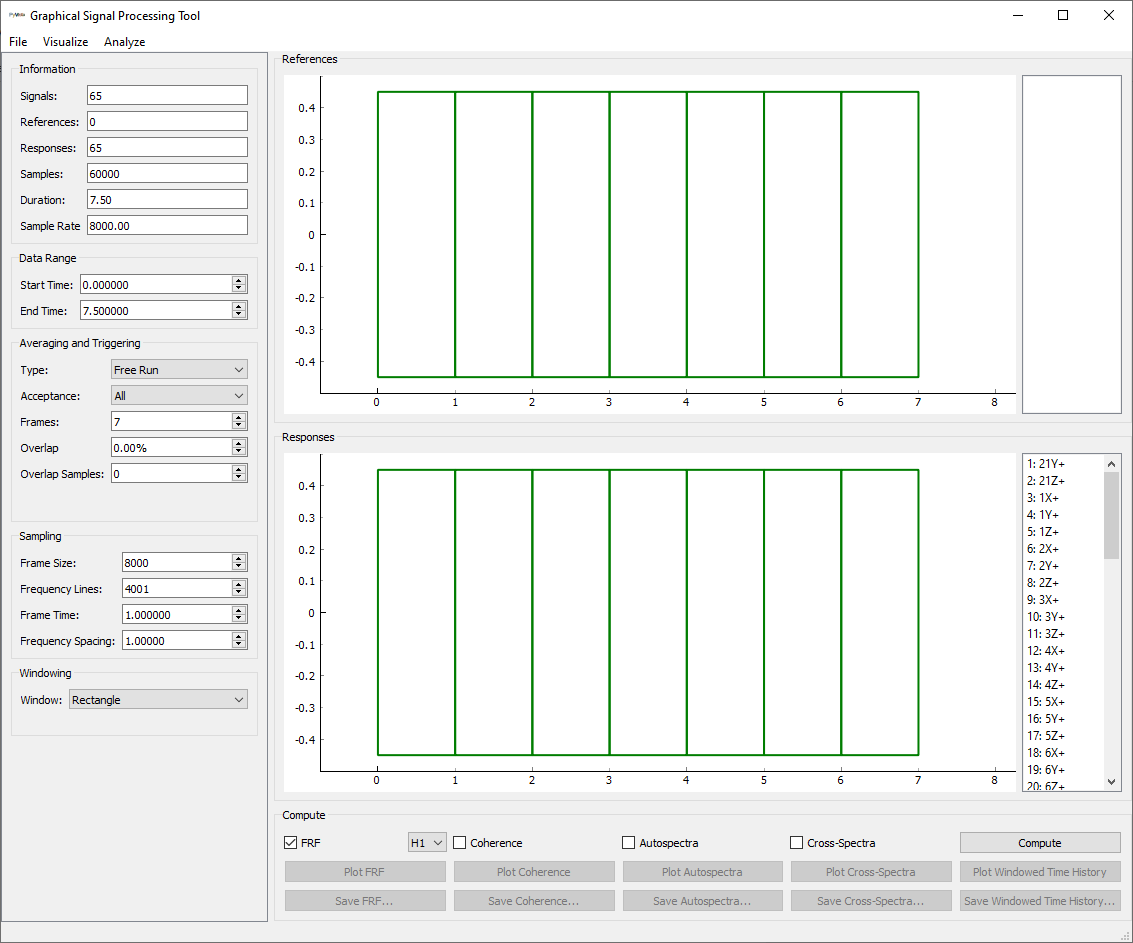
SignalProcessingGUI
that initially appears for our test case.
Let’s first explore the SignalProcessingGUI Window. On the top left is a set of Information
about the signals that are loaded. We see there are 65 signals total, of
which 0 are references and 65 are responses (we will fix this shortly). There
are 60000 samples for a duration of 7.5 seconds, and the sample rate is 8000 Hz.
Below the information we have the Data Range. This allows us to select a range
over which the computation will be performed. This is useful for targetting
portions of an environment, or for discarding portions of data that are not yet
at steady state.
Below that are the Averaging and Triggering settings. This allows users to
specify when the frames occur in the signal, either by setting them up every
so many samples, or detecting some kind of trigger signal to use to locate the
measurement frames.
Below that are the Sampling options, where the frame length is specified.
Finally, the last options are for Windowing. Certain windows may have extra
parameters that will appear in this box, for example, the decay of an exponential
window.
In the center of the window, we see two plots that are currently empty except
for some green boxes. These green boxes represent the measurement frames in
the signal. Currently no signals are plotted, because we have not selected any
signals from the lists on the right side of the window. There are currently no
signals listed in the References list; all are currently in the Responses
list. Signals can be moved from reference to response and vice versa by
double-clicking the signal name in the list on the right side. Note also that
when a signal is selected, it will be shown in the respective plot.
Finally, on the bottom right corner of the window, we have signal processing
computations that can be performed. The check boxes denote which functions
to compute when the Compute button is pressed. Once a function is computed,
it can be plotted or saved to a file.
There are also menus at the top of the window that contain additional functionality.
The File menu allows data to be loaded directly from the disk. The
Visualize menu allows the data to be sent to the transient or deflection shape
plotters once a geometry is loaded (or assigned via code as we have done).
The Analyze menu allows data to be sent to curve fitting software,
though these are currently disabled until frequency response functions have been
computed.
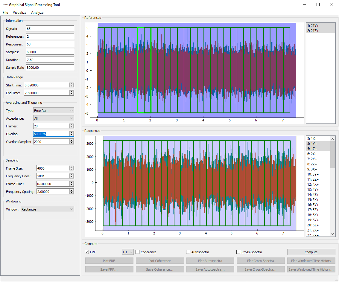
To start with, we will send our forces, which are the first two signals in the responses list to the references list by double-clicking them. We should now see those signal as a reference in the top list and plotted in the top plot. Let’s also select the drive point responses in the bottom list (only single click, not double click) so they are plotted in the bottom plot.
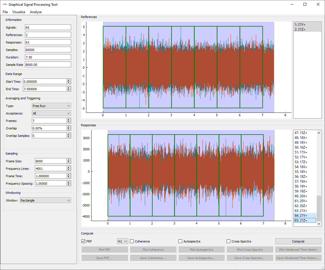
SignalProcessingGUI
with reference signals moved to the References window by double-clicking them.
After this step, we should see that the References box in the Information
section shows 2 and the Responses box shows 63.
The next thing we will check is our sampling. We set up our signals to
provide 2 Hz frequency spacing, so we can set that in the Frequency Spacing
box in the Sampling section of the window. Note that this will automatically
adjust all other properties that are determined by the frequency spacing. For
example, the Frame Time has adjusted automatically to 0.5 seconds. You will
also see that the displayed frames on the plots have changed lengths, being now
half the size they were before.

SignalProcessingGUI
with sampling set to 2 Hz frequency spacing.
Note that since we have started from zero velocity and displacement, there may
be some start-up transients in the signal. If we zoom in the the start of the
Responses plot, we can see that it takes approximately 0.01 seconds to get
to a steady-state level. We can therefore set the Start Time in the
Data Range section of the window to 0.02 seconds, just to be sure we’re
at steady state. We could also perform this operation by dragging the left side
of the blue region in the plot to the position that we desire. After performing
this operation, we should see that all the green boxes have slide to the right,
starting at the position specified by the Start Time. We also see that we
have lost a measurement frame that no longer fits at the end of the signal;
can be seen in the Frames box in the Averaging and Triggering section,
which has changed from 15 to 14.
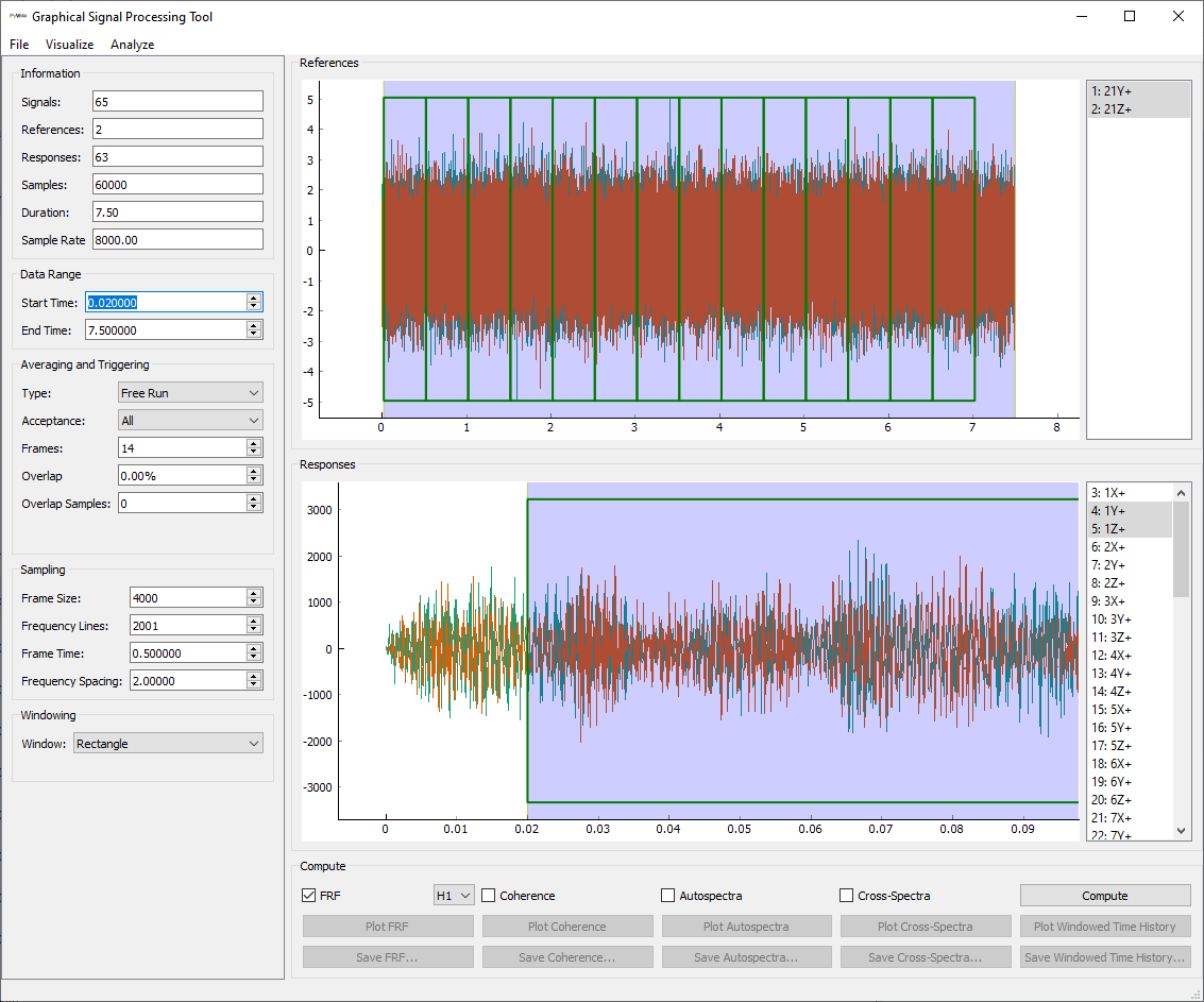
SignalProcessingGUI
with the start time set correctly.
We will then adjust the overlap between measurement frames. We will set the
Overlap box in the Averaging and Triggering section of the window to
50.00%. We can see that the green boxes are now overlapping. This overlap
can be easier to see if you hover the mouse over one of the boxes, which will
cause it to highlight.
SignalProcessingGUI
with the overlap set to 50% and a single measurement frame highlighted.
The last setting we will set is the Window in the Windowing section
of the window. We will specify a Hann window (known as a Hanning window in
some vibration literature).
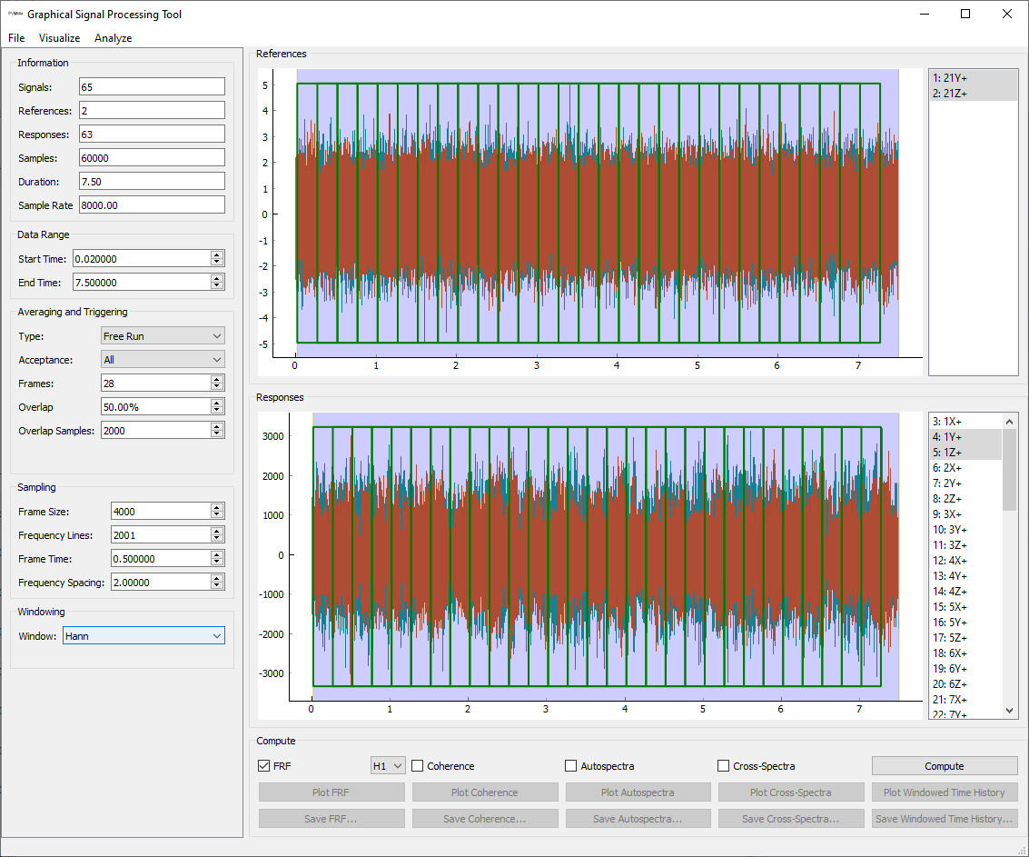
SignalProcessingGUI
with the window set to Hann.
Finally we can compute the frequency response functinos. We ensure that the
check box next to FRF is selected in the Compute section of the window.
Additionally, we will compute the coherence by checking the Coherence
checkbox. We can then press the Compute button. When the computations are
finished, the buttons under the computed functions will be enabled, and we can
plot them.
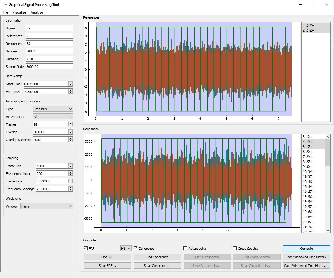
SignalProcessingGUI
with the functions computed.
Clicking the Plot FRF or Plot Coherence buttons will cause those
plots to appear in a GUIPlot window.
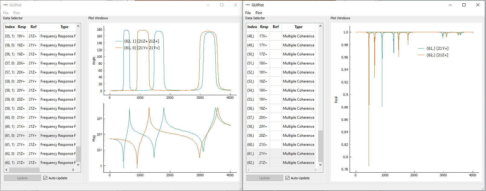
Drive point frequency response function and multiple coherence computed by
SignalProcessingGUI
Data can be saved from the
SignalProcessingGUI
window by clicking the Save FRF... button, and can be re-loaded into SDynPy
using the
sdpy.data.load function.
In this case, we have saved the file into the current working directory as
frfs_signalprocessinggui.npz so we can load it using
frfs_spgui = sdpy.data.load('frfs_signalprocessinggui.npz')
Plotting Deflection Shapes
While we could pass these shapes into the modal fitters in SDynPy, the lower-effort
solution could be to simply examine the deflection shapes to pick out approximate
frequencies and deflection shapes of the structure. We can easily plot
deflection shapes using the
plot_deflection_shape
method of the Geometry class.
This method accepts a set of spectral data, such as frequency response functions.
However, because the
DeflectionShapePlotter
will attempt to map responses onto the geometry, we will not be able to plot
multiple references simultaneously, as this will result in frequency response
functions with identical response coordinates. Because our frequency
response function arrays are already shaped as (num_response,num_reference),
we can simply index into the last dimension of the array to select single-reference
frequency response functions.
In [66]: geometry.plot_deflection_shape(frfs_spgui[:,0])
Out[66]: <sdynpy.core.sdynpy_geometry.DeflectionShapePlotter at 0xXXXXXXXXXXX>

In [67]: geometry.plot_deflection_shape(frfs_spgui[:,1])
Out[67]: <sdynpy.core.sdynpy_geometry.DeflectionShapePlotter at 0xXXXXXXXXXXX>
DeflectionShapePlotter
interactive deflection shape viewer from reference 1
DeflectionShapePlotter
interactive deflection shape viewer from reference 2
These windows are similar to those of the transient plotter in that the cursor
at the bottom of the window can be used to select the frequency at which the
deflection shape is animated. The << and >> buttons step left or right
by a single frequency line. The Play and Stop buttons start and stop
the animation, respectively. Complex display, shape scaling, and animation
speed can be adjusted in the Shape menu.
Note that you can directly send your frequency response functions to the
DeflectionShapePlotter
through the Visualize menu of the
SignalProcessingGUI
Fitting Modes to Frequency Response Functions
Particularly when performing experimental modal analysis, we will generally wish to fit modes to the frequency response functions. Let’s look at some of the tools available to fit modes to frequency response functions in SDynPy.
PolyPy
PolyPy is a polynomial-based curve fitter, and analysis typically occurs in two parts. In the first part, users specify frequency bands of interest as well as the different polynomial orders to solve. PolyPy will then solve the polynomial at those orders and produce a stability diagram, which can help identify real modes from computation modes. In the second part, users will pick modes from the stability diagram to use in the final mode set. PolyPy will reconstruct frequency response functions from that set of modes, which can be compared against the original frequency response functions to judge adequacy of fit.
PolyPy is an implementation of PolyMax
[4].
It is the most mature curve fitter in SDynPy. It can be run either via code or
via graphical user interface. We will focus on the graphical user interface
version of the code here, which is accessed via the
PolyPy_GUI class. The class
initializer accepts the frequency response functions as an input. Again we can
assign geometry to the fitter for shape plotting so we don’t have to load it
from disk.
polypy = sdpy.PolyPy_GUI(frfs_spgui)
polypy.set_geometry(geometry)
Alternatively, PolyPy_GUI
can be run from the Analyze menu of the
SignalProcessingGUI
window to stay in graphical user interfaces. Any geometry loaded into
SignalProcessingGUI
will automatically be sent to the
PolyPy_GUI.
The initial PolyPy_GUI window
is shown below.
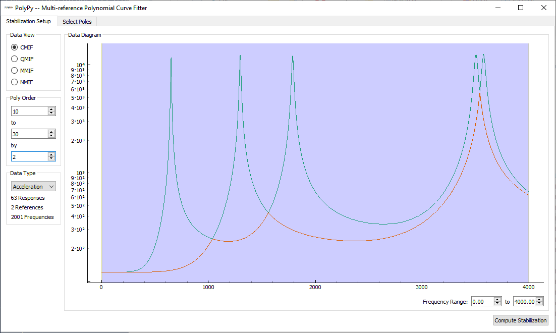
Initial window of the PolyPy_GUI
We can see that the window is separated into two tabs, corresponding to the two
main parts of the PolyPy workflow. The first tab is Stabilization Setup,
which allows the user to select the parameters of the stability calculation.
The second tab is Select Poles where the final mode set is selected.
Starting with the Stabilization Setup tab, we see that there is a main plot
in the Data Diagram section of the of the window. This shows the mode
indicator function indicated by the selection in the Data View section
of the window; currently, the Complex Mode Indicator Function is shown.
The polynomial orders that will be computed in the stability diagram are specified
in the Poly Order section of the window. Users can specify the range of
polynomial orders to compute, as well as the step size. The current values of
10, 30 and 2 will result in computation of polynomial orders 10, 12,
14, … , 26, 28, and 30. The Data Type portion of the window allows
specification of the type of frequency response function that is being analyzed.
In our case, our frequency response function is an Acceleration over Force
frequency response function, so we can leave the default Acceleration
selection.
Below the main plot in the Data Diagram portion of the window, the
Frequency Range can be specified. The
PolyPy_GUI implementation in
SDynPy allows analyzing multiple frequency ranges separately and then combining
the final selected modes into a single set. We will demonstrate this capability
here.
We will set the frequency range of the analysis to initially target the first
three modes of the system. We can do this by adjusting the values of the
Frequency Range boxes, or by dragging the edges of the blue region of the
plot.
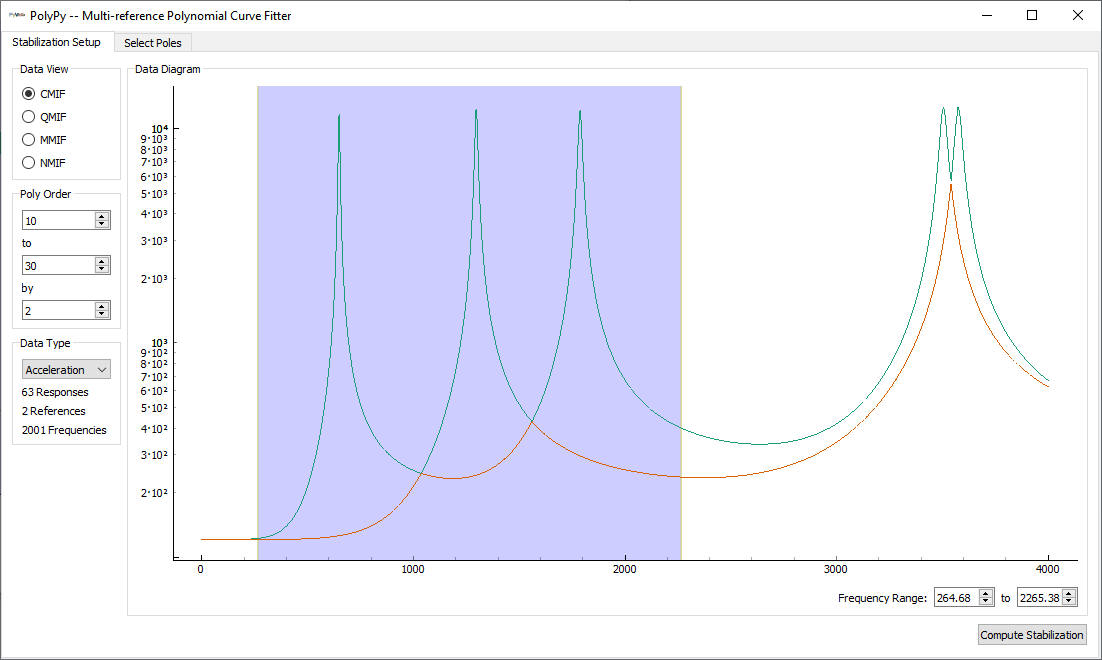
Selecting the first analysis region in
PolyPy_GUI
We can then click the Compute Stabilization button to tell PolyPy to
compute the stabilization diagram for these parameters. Progress for these
computations is shown in the console window. After the computations
are performed, the PolyPy_GUI
will automatically proceed to the Select Poles tab.
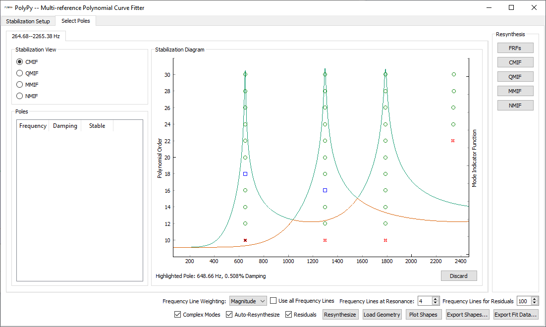
Initial stability diagram for the first analysis region in
PolyPy_GUI
Prominent in this tab is the stabilization diagram, shown in the
Stabilization Diagram portion of the window. The stabilization diagram
consists of a mode indicator function (similarly chosen by selecting an entry
in the Stabilization View portion of the window) overlaid with various
markers that represent poles of the system (frequency and damping ratio). The
color and shape of the poles determine how stable the pole is. Stability is
computed by how much or little the pole changes as different polynomial orders
are computed. A real mode will tend to remain unchanged if different order
polynomials are solved. Computational poles, on the other hand, will tend to
vary as different orders are solved. In PolyPy, a red X signifies an instable
pole, a blue triangle signifies that the frequency has stabilized, a
blue square signifies that the frequency and damping have stabilized, and a
green circle signifies that the frequency, damping, and participation factor
of the mode has stabilized. Generally, we should only select green circles in
the stabilization diagram, preferably at an order where the symbol has been
green for a few orders.
In the PolyPy_GUI, poles are
selected by clicking on the markers on the stabilization diagram. When hovering
the mouse over a marker, PolyPy_GUI
will report the frequency and damping of that pole in the bottom left corner of
the plot window. When selected, the marker will turn a solid color, and the
pole will be reported in the table in the Poles section of the window.
If for whatever reason the stabilization diagram is not useful (perhaps the
wrong polynomial orders were specified) users can click on the Discard
button, which will delete the current stabilization diagram. The user can then
proceed to the initial tab and select new parameters and recompute the
stabilization diagram.
As modes are selected, the PolyPy_GUI
will attempt to resynthesize frequency response functions from the selected shapes.
Options for performing this resynthesis are at the bottom of the window.
The Frequency Line Weighting specifies how the frequency lines are weighted
when computing mode shapes. If Magnitude is selected, larger magnitude
frequency lines are weighted more heavily in the computation. If Uniform
is selected, all frequency lines are considered equally. Users can also specify
which frequency lines are used in the computation by adjusting the
Frequency Lines at Resonance and Frequency Lines for Residuals parameters.
The former specifies how many frequency lines around each pole are used for
computing mode shapes. This can be useful for analysis with relatively high
noise floors, where the noise in the valleys between the peaks could contaiminate
the estimation of the mode shape. The latter specifies how many frequency lines
at the beginning and end of the frequency range get included in the mode shape
computation when residuals are computed. If all frequency lines are desired,
users can simply check the Use all Frequency Lines checkbox.
Users can switch between real and complex modes by unchecking or checking the
Complex Modes checkbox. If the Auto-Resynthesize checkbox is checked,
PolyPy_GUI will resynthesize
frequency response functions after each mode is selected. This can be useful
for smaller systems to see the immediate effect of adding a specific mode; however,
this can slow the analysis down for larger datasets where it can take a non-negligable
amount of time to resynthesize shapes. If the Auto-Resynthesize checkbox
is not checked,frequency response functions can be manually resynthesized by
clicking the Resynthesize button. Finally, the use of residuals in mode shape
computation can be selected by clicking the Residuals checkbox.
To see the resynthesized frequency response functions compared to the original
ones, users can click on the buttons in the Resynthesis portion of the
window. This will plot the frequency response functions or mode indicator
functions in a separate window. These plots will be updated automatically
each time frequency response functions are resynthesized.
To start our analysis, let’s click the CMIF button to bring up a the
resynthesized complex mode indicator Function plot. Initially, just one set of
data will be plotted as we currently do not have any modes selected on the
stability diagram. Ensure both singular values of the CMIF are selected in the
GUIPlot window. Let’s click the
Use all Frequency Lines checkbox as well, and deselect the Complex Modes
checkbox.
Now we will start selecting markers in the stabilization diagram. Users should note that the resynthesized CMIF should be updated as additional modes are selected. Ensure that green circle markers are selected for each of the three main peaks in the CMIF. We will not select one of the green circles around 2340 Hz, as there is no peak in the CMIF to indicate a real mode at that frequency.
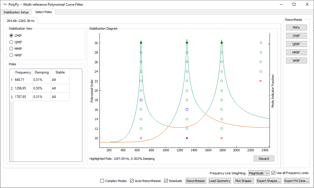
Stability diagram for the first analysis region with three modes selected
PolyPy_GUI
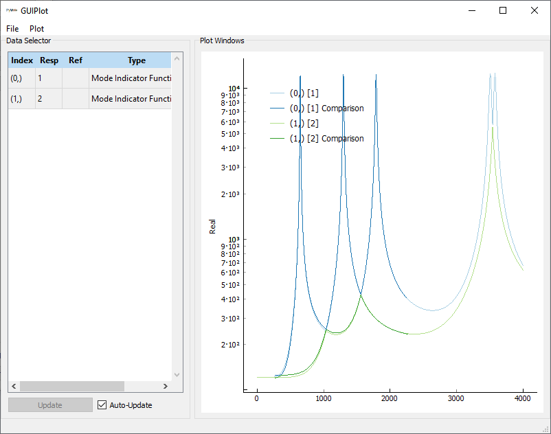
Resynthesis of the CMIF using the fit modes and residuals from the first frequency region compared to CMIF computed from the original frequency response functions.
Given that this is a purely synthetic dataset, very good fits to the data should be achievable, as shown in the previous figure up to 2200 Hz. However, we still have the peaks between 3000 and 4000 Hz to fit, so let’s do that now.
Return to the Stabiliziation Setup tab (do not discard the previous
stabilization diagram by pressing the Discard button!). We will now
set up an analysis targetting the missing modes. We can adjust the blue region
from approximately 3000 to 4000 Hz to target these peaks.
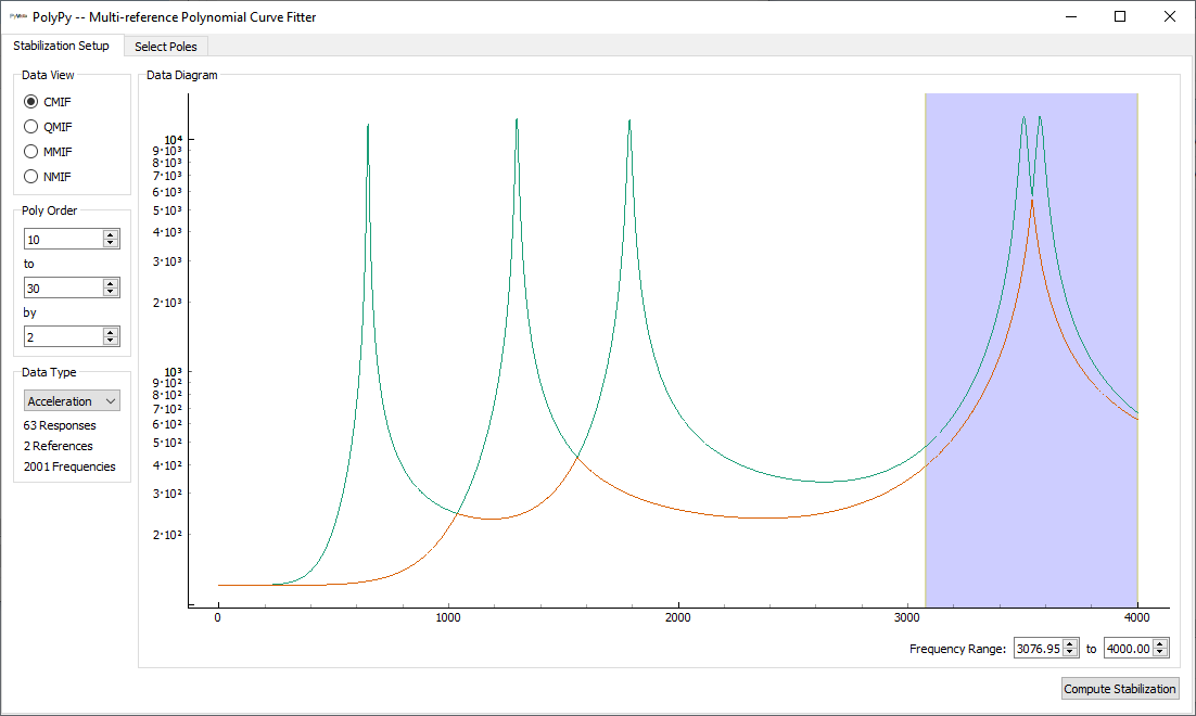
Selecting the second analysis region in
PolyPy_GUI
We can then again click the Compute Stabilization button, which will
bring us again to the Select Poles tab. Note here that we now have two
sub-tabs on this window, each representing a different frequency range that
we analyzed. The first region is on the 264.68--2265.38 Hz tab, and the
second is on the 2076.95--4000.00 Hz tab. Note the exact values will differ
depending on the exact frequency range selected.
We can then continue selecting modes in this frequency range. We will pick the green circles corresponding to the strong peaks in the CMIF. As we pick markers in this frequency range, we should see the modes be combined with the modes from the previous region when the resynthesis is occuring.
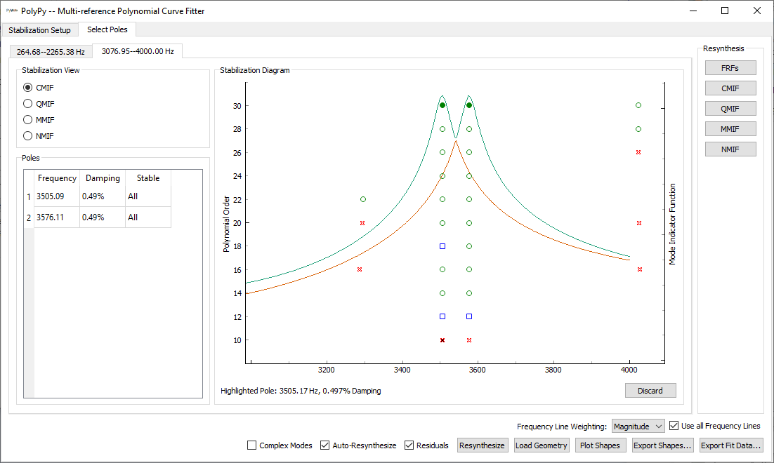
Stability diagram for the second analysis region with two modes selected
PolyPy_GUI
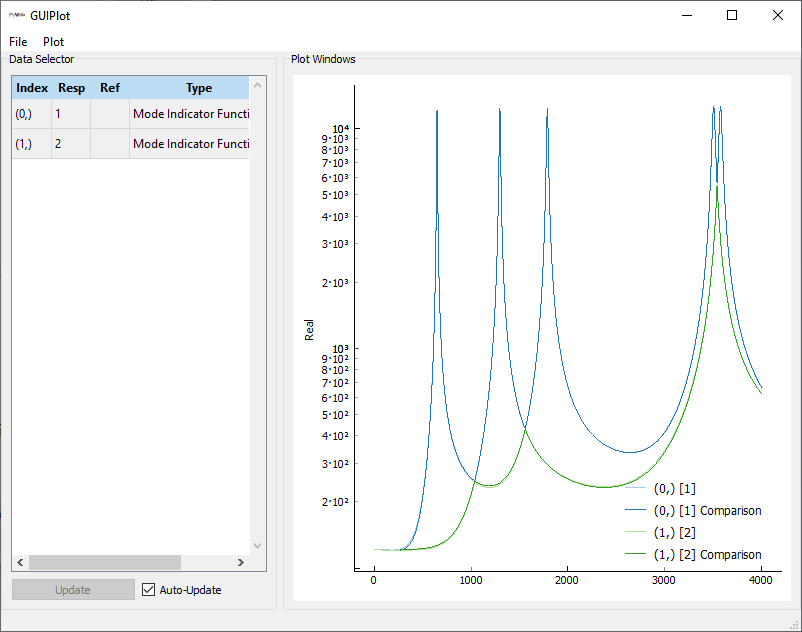
Resynthesis of the CMIF using the fit modes and residuals compared to CMIF computed from the original frequency response functions.
Clearly we have achieved very good fits, which is expected due to the synthetic data set.
With modes fit, we can plot the mode shapes by selecting the Plot Shapes
button. Note that had we not assigned geometry to the
PolyPy_GUI
using its
set_geometry
method, we would need to first load geometry using the Load Geometry button
prior to being able to plot shapes. An example mode shape is shown below.

Mode shape of the beam computed from PolyPy animated on the geometry.
We will then save the shape files to disk by clicking the Export Shapes...
button. We will save the shapes to a file shapes_polypy.npy. If we also
wanted to save the resynthesized frequency response functions, we could click
the Export Fit Data... button, which saves a much more complete data set
to disk.
Synthesize Modes and Correlate (SMAC)
The second curve fitter available in SDynPy is Synthesize Modes and Correlate
(SMAC) [3]. SMAC is a modal-filter based curve fitter.
While it is not as polished as the PolyPy curve fitter, it can often provide
better fits than PolyPy if the data quality is not as good. Simlar to PolyPy,
SMAC can be run both via code or via graphical user interface. We will
demonstrate the latter here using the
SMAC_GUI class. Again, we can
assign geometry directly to the SMAC_GUI
object so we don’t need to load from disk.
smac = sdpy.SMAC_GUI(frfs_spgui)
smac.geometry = geometry
Similarly to PolyPy, the SMAC_GUI
is separated into different tabs representing different portions ofthe workflow.
The first tab, Pseudoinverse is where the pseudoinverse of the frequency
response function matrix is performed. At this stage, we need to specify the
frequency range we are working over, as well as the data type, and whether
or not complex modes will be fit. To keep a similar analysis to that in PolyPy,
we will choose Normal Modes rather than Complex Modes. We will set the
Frequency Range from 260 to 4000 Hz, and we will keep the Data Type
as Acceleration.
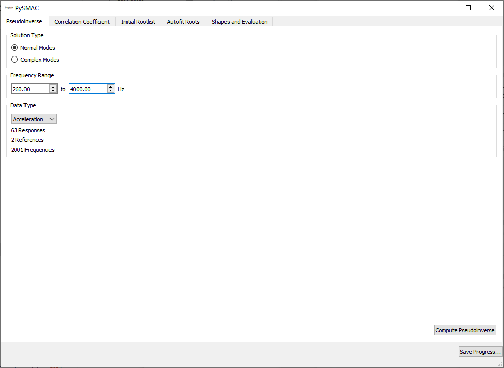
When this is set correctly, we can press the Compute Pseudoinverse button
to perform the computation and move to the next tab.
The next tab is the Correlation Coefficient tab. SMAC finds modes by comparing
what a mode should look like to what the frequency response functions do look
like to identify where modes are in the frequency response function. It uses
the correlation coefficient to make these comparisons. Where the correlation
coefficient approaches 1.0, one can be reasonably certain a mode is present.
Where the correlation coefficient is far from 1.0, a mode is not likely present.
SMAC generally guesses a large number of frequencies and damping values, finds
where the correlation coefficient is high, and then narrows in to converge on a
mode. The Correlation Coefficient tab sets up the initial set of guesses
that SMAC makes. The frequency resolution of the initial guesses is set via the
Frequency Spacing value, and the Lines to use in Correlation Computation
value specifies how many frequency lines around each frequency guess get used
to compute the correlation coefficient. Also specified is an initial guess for
damping. In the present case, we know the damping because we specified it to be
0.5%. In a real situation, we generally would not know this information a priori.
Therefore we will leave this page with default values.
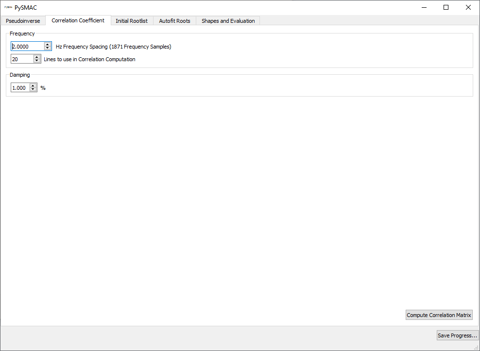
We can then click the Compute Correlation Matrix button to proceed to the
Initial Rootlist tab. This tab shows a mode indicator function in the
upper plot and the correlation coefficient at each frequency guess in the lower
plot. It will attempt to initially automatically select peaks in the correlation
coefficient plot higher than the value specified by the Minimum Coefficient
box, and populate the Root List on the left side of the window. We can
see for this perfect synthetic data set,
SMAC_GUI has made very good
initial guesses for our modes, even with 1% damping specified when the true
damping should be 0.5%. The Root List also reports the current correlation
coefficient, which is near 1. If initial guesses at roots were not identified
successfully, the user can click on the Correlation Coefficient plot to place
additional initial guesses. Also, if erroneous initial guesses were placed,
the user can select the row in the Root List table and click the Delete
button.
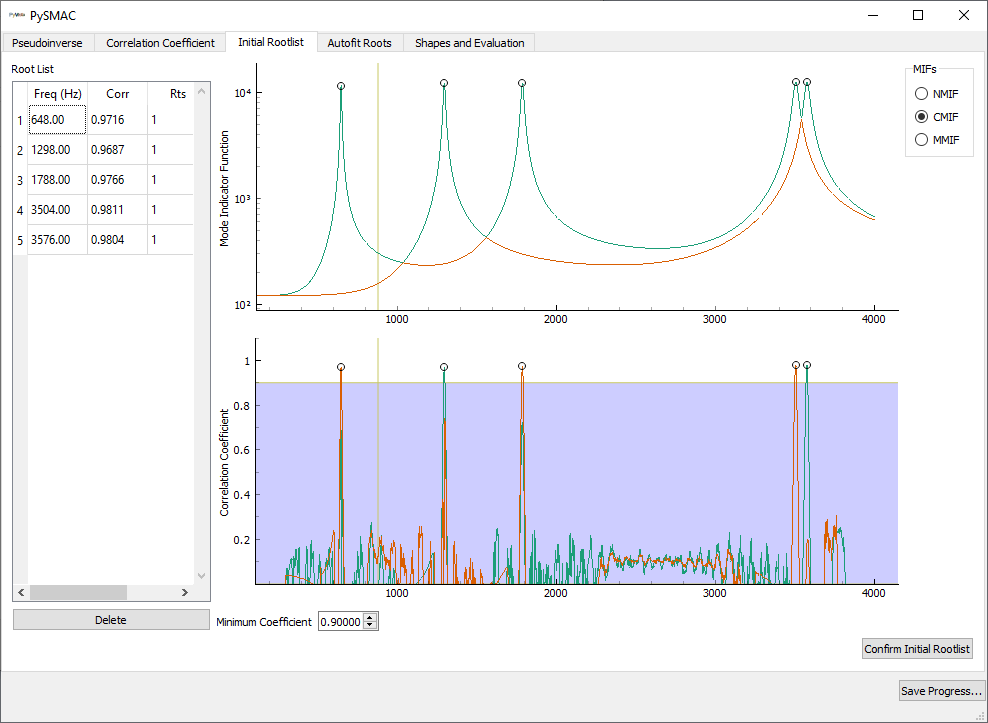
Clicking the Confirm Initial Rootlist button proceeds to the Autofit Roots
tab. This tab sets up the optimizer that will converge to the frequency and
damping that gives the highest correlation coefficient from the initial guesses
obtained on the previous tab. Generally the default values work well for this,
though users may want to tighten or loosen the convergence tolerances depending
on their goals.
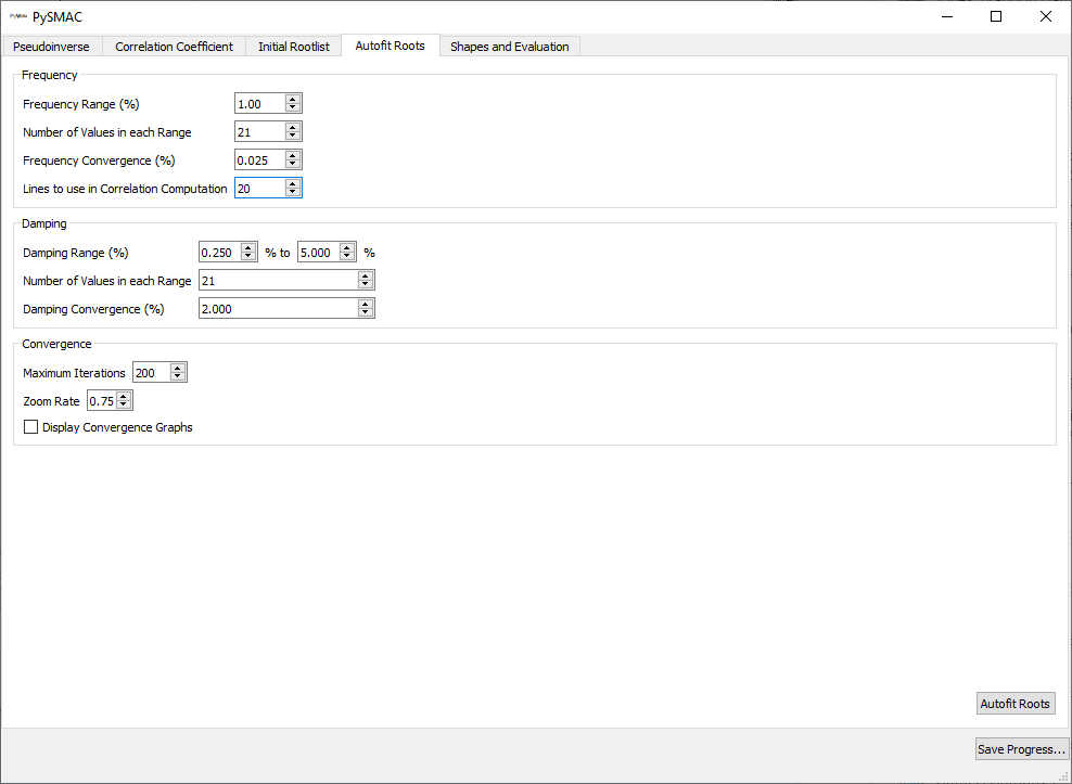
Clicking the Autofit Roots button will start the optimizer. Progress is
reported in the console window. If a root diverges, SMAC will discard it.
Similarly, if a root converges into another root, SMAC will discard one of them
to only keep one root. When the optimizer has finished,
SMAC_GUI will proceed to the final
Shape and Evaluation tab.
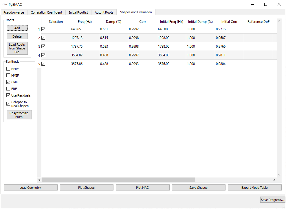
The Shape and Evaluation tab shows the final root list table, consisting of
the frequency and damping values that the optimizer converged on. Modes can
be selected or deselected from the final root set by checking or unchecking the
checkbox in the Selection column of the table. If additional modes occur in
the data that were not captured in the initial root list, they can be added
manually by clicking on the Add button. Likewise, if roots are found to
be incorrect, they can be selected in the table and deleted by pressing the
Delete button. Resynthesis of frequency response functions or mode indicator
functions can be performed by checking the boxes in the Synthesis area of
the windows. Additional options for using residuals or collapsing complex
modes to real modes can also be found there. Clicking the Resynthesize FRFs
button will trigger the resynthesis.
Clicking the Resynthesize FRFs button will also bring up a
GUIPlot window plotting the
selected resynthesis quantities.
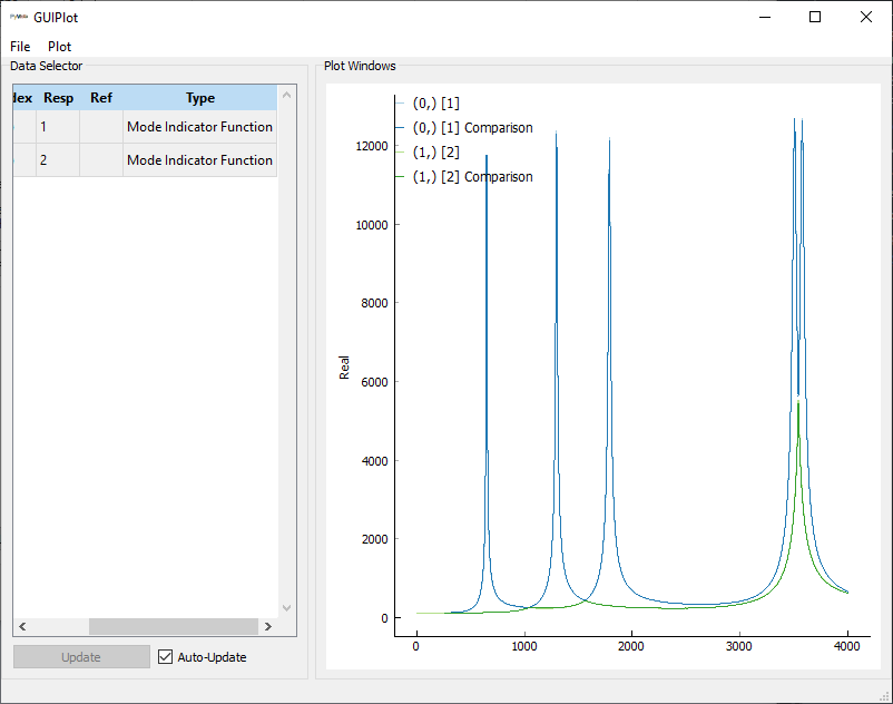
Resynthesis of the CMIF using the fit modes and residuals compared to CMIF computed from the original frequency response functions.
The SMAC_GUI Add button
brings up the Add Root dialog box. We will cover this briefly, as its usage
can be somewhat unintutive. In essence, the user is acting as the optimizer
while SMAC solves for the correlation coefficient over ranges of frequency
and damping values.
When the Add Root dialog appears, the initial frequency range is set to the
entire frequency range, and the initial damping range is set to the parameters
used in the Autofit Root tab. The number of samples across the frequency
and damping axes are also taken from the values on this tab, though they can
be changed. The top image in the dialog box shows a 2D correlation coefficient
plot where lighter colors correspond to a larger correlation coefficient.
The goal is to zoom in on the image (tightening frequency and damping tolerances)
until we converge on a peak in the correlation coefficient, which should
correspond to a mode of our system.
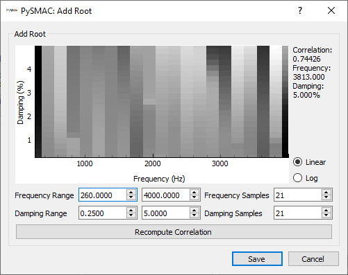
Add Root dialog showing the initial optimization range spanning the entire frequency range.
Normally, we will know approximately the frequency range in which we are
targetting a mode, either from a peak in a mode indicator function or a poor
frequency response function resynthesis in a given frequency band. While in the
present case, SMAC has converged on all modes of the system in the bandwidth,
we will pretend that it has missed the fifth mode. From the CMIF, we can see
that the fifth mode should be somewhere between 3550 and 3600 Hz, so we can
set that as th initial frequency range and click the Recompute Correlation
button.
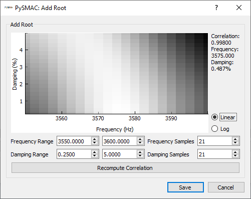
Add Root dialog after setting an initial frequency range and recomputing the correlation coefficient
There clearly is a peak in this region, given the large swath of white
color on the image. We can see in the text on the right side of the window that
the maximum correlation in the image is currently 0.998 with a frequency at
3575 Hz and a damping value of 0.487%. However, it can be difficult to identify
this position on the image due to the limited contrast available using the
linear colormap. If we instead switch the colormap from Linear to Log,
we will see a much sharper peak that we can zoom into.
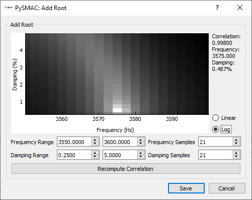
Add Root dialog after setting an initial frequency range and recomputing the correlation coefficient, visualized with logarithmic colormap
Clearly this Log view of the correlation coefficient more accurately
pin-points the location of the peak correlation coefficient. In general,
the Linear colormap is more useful when performing rough finding of peaks
in the data, and the Log colormap is more useful when performing the final
“hone in” on the peak.
To converge on the peak, we can simply zoom in on the image and click the
Recompute Correlation button. We can do this until we reach our desired
convergence tolerance. Note, however, that eventually we will reach numerical
precision and the colormap will break down. If this happens, simply zoom out
a bit and Recompute Correlation.
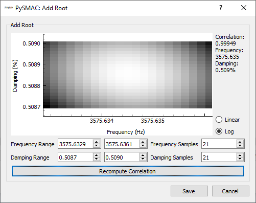
Add Root dialog after converging on a frequency and damping.
Clicking the Save button on the dialog will then close the dialog and add
the mode to the table. We can see that this mode has a slightly higher
correlation coefficient than the original mode found by the optimizer, so we
could select that row and press the Delete button to ensure that the mode
isn’t included twice. Again we can plot the mode shapes by pressing the Plot Shapes
button (be sure to click the Resynthesize FRFs button first, which will
create the shapes, otherwise a dialog will appear telling you the shapes have not
been created yet).
Finally we can write the shapes to disk. We will then save the shape files to
disk by clicking the Save Shapes
button. We will save the shapes to a file shapes_smac.npy.
Comparing Modes
In many modal analysis workflows we wish to compare shapes to each other. For example, we may wish to compare shapes from a finite element model to those from a test. Or perhaps we may wish to compare two sets of shapes from a model that has varying parameters. SDynPy offers several ways to easily compare modes.
First, let’s load the modal data from the previous modal analyses. We will
use the sdpy.shape.load
function targetting the file names from the previous analyses. If the files
are not in the current working directory, a full path will need to be provided.
shapes_polypy = sdpy.shape.load('shapes_polypy.npy')
shapes_smac = sdpy.shape.load('shapes_smac.npy')
To compare modes, we often need to first figure out which modes in each dataset correspond to one another. Especially if closely spaced modes exist, there may be mode order changes, so we cannot always compare the first mode in the first data set with the first mode of the second. Especially when comparing model to test data, there may be rigid body modes from the model that were not measured in the test. Mode correspondences are often assigned via shape, often using a metric such as the Modal Assurance Criterion (MAC) matrix.
SDynPy can construct a MAC matrix easily using the
sdpy.shape.mac function. The matrix
can be plotted using the
sdpy.matrix_plot
function.
# Compute MACs
mac_polypy = sdpy.shape.mac(shapes,shapes_polypy)
mac_smac = sdpy.shape.mac(shapes,shapes_smac)
# Create a figure
fig,ax = plt.subplots(1,2,num='MAC Matrices',sharey=True,sharex=True)
# Plot the PolyPy MAC
sdpy.matrix_plot(mac_polypy,ax=ax[0])
ax[0].set_ylabel('FEM Shapes')
ax[0].set_xlabel('PolyPy Shapes')
# Plot the SMAC MAC
sdpy.matrix_plot(mac_smac,ax=ax[1])
ax[1].set_ylabel('')
ax[1].set_xlabel('SMAC Shapes')
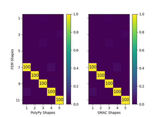
MAC between fit shapes and finite element shapes.
The frequency and damping ratios are also often compared. The
sdpy.shape.shape_comparison_table
function is useful for this. We can pass in two sets of shapes to see the
tabulated differences in the parameters. First we will need to extract the
shape correspondences.
polypy_correspondences = np.where(mac_polypy > 0.9)
smac_correspondences = np.where(mac_smac > 0.9)
Then we can print the mode tables. We will adjust the formatting of the percent errors to give more decimal places, as the default will only plot one decimal place, resulting in all frequencies having 0.0% error.
print(sdpy.shape.shape_comparison_table(
    shapes[polypy_correspondences[0]],
    shapes_polypy[polypy_correspondences[1]],
    percent_error_format='{:0.3f}%'))
This results in printing the following table.
Mode  Freq 1 (Hz)  Freq 2 (Hz)  Freq Error  Damp 1  Damp 2  Damp Error  MAC
   1       648.56       648.71     -0.024%   0.50%   0.51%     -1.064%  100
   2      1297.12      1296.95      0.014%   0.50%   0.50%     -0.307%  100
   3      1787.81      1787.95     -0.008%   0.50%   0.51%     -2.028%  100
   4      3504.98      3505.09     -0.003%   0.50%   0.49%      1.672%  100
   5      3575.61      3576.11     -0.014%   0.50%   0.49%      2.010%  100
The identical analysis is performed for the SMAC dataset.
print(sdpy.shape.shape_comparison_table(
    shapes[smac_correspondences[0]],
    shapes_smac[smac_correspondences[1]],
    percent_error_format='{:0.3f}%'))
Which results in
Mode  Freq 1 (Hz)  Freq 2 (Hz)  Freq Error  Damp 1  Damp 2  Damp Error  MAC
   1       648.56       648.65     -0.014%   0.50%   0.55%     -9.198%  100
   2      1297.12      1297.13     -0.001%   0.50%   0.51%     -2.900%  100
   3      1787.81      1787.75      0.003%   0.50%   0.53%     -6.121%  100
   4      3504.98      3504.82      0.005%   0.50%   0.49%      2.564%  100
   5      3575.61      3575.63     -0.001%   0.50%   0.51%     -1.750%  100
We can see that SMAC has perhaps identified frequencies more accurately, but was less accurate on the damping estimates. Note that these are not general rules and likely depend on the parameters selected in each curve fitting tool. Note that both curve fitters have identified the modes very accurately.
While the MAC can give a rough idea of how correlated pairs of shapes are, it
does not give an intuitive view of how the shapes are different. For this, we
would often like to plot the shapes on top of one another. We can also do this
easily in SDynPy with the
sdpy.Geometry.overlay_geometries
and
sdpy.shape.overlay_shapes
functions.
Note that the
sdpy.shape.overlay_shapes
function will automatically call the
sdpy.Geometry.overlay_geometries
functions, so if we are comparing shapes, we only need to call the latter function.
We simply give the function a set of geometries and a set of shapes to overlay,
and we can additionally specify colors to override so we can identify which is
which. Because the fit shapes and finite element shapes share the same geometry,
we simply pass it twice.
# Overlay shapes
overlaid_geometry,overlaid_shapes = sdpy.shape.overlay_shapes(
    (geometry,geometry),
    (shapes[polypy_correspondences[0]],shapes_polypy[polypy_correspondences[1]]),
    color_override=[1,7])
# Plot the overlaid shapes
overlaid_geometry.plot_shape(overlaid_shapes)
Finite element (green) and fit (blue) shapes overlaid.
Adding Another Beam
Let’s make our system more complicated by adding an additional beam. We can demonstrate some of SDynPy’s more advanced features by combining the two structures together. This beam will be half as long as the previous beam and connect at a right angle to the end of the first beam.
system_2,geometry_2 = sdpy.System.beam(
    length = 0.1, # Meters
    width = 0.01, # Meters
    height = 0.005, # Meters
    num_nodes = 11,
    material='steel')
We will modify the geometry of this second beam by rotating its coordinate system. We will also change the color of the traceline so it is more distinguishable from the initial beam.
geometry_2.coordinate_system.matrix[0,:3,:3] = np.array([[0,1,0],
                                                         [0,0,1],
                                                         [1,0,0]])
geometry_2.traceline.color = 7
If we plot the geometry, we can now see that it is oriented 90 degrees to the
original geometry. We can use the
sdpy.Geometry.overlay_geometries
function to quickly produce a combined geometry which to plot. We will also have
the system return a node_id_offset, which we can use to offset the degrees
of freedom of our systems so they remain consistent with the geometry. This is
needed because the
sdpy.Geometry.overlay_geometries
function offsets the node numbers so there are no conflicts between the two
geometries.
# Overlay geometry and plot
combined_geometry,node_id_offset = sdpy.Geometry.overlay_geometries(
    (geometry,geometry_2),
    return_node_id_offset=True)
# Plot the combined geometry
combined_geometry.plot()
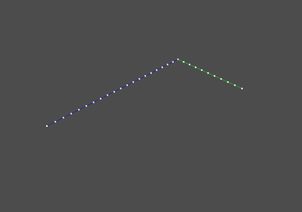
Geometry of the two-beam system.
Now let’s think about combining the systems. First, let’s add some damping to
the systems. We saw previously that we had some issues with the undamped systems
not being equivalent to shapes, as well as having potentially infinite displacement.
We can add some approximate damping to the
system such that when a modal transformation is performed, it will result in
modal damping. The System object
has an
assign_modal_damping
method that is useful for doing this.
damped_system = system.copy()
damped_system.assign_modal_damping(0.005)
damped_system_2 = system_2.copy()
damped_system_2.assign_modal_damping(0.005)
With damping added, we can concatenate the systems together using the
concatenate class
method of System. Note that this
does not actually attach either structure to the other. It simply puts them in
the same System object. If we
examine the system matrices, we will see there is no coupling between any
degrees of freedom on the first beam to the second beam. Note that the
concatenate
function accepts the node_id_offset from the
sdpy.Geometry.overlay_geometries
function.
combined_system = sdpy.System.concatenate((damped_system,damped_system_2),
                                          node_id_offset)
# Plot the combined system matrices
fig,ax = plt.subplots(2,2,num='Combined System Matrices',figsize=(8,6))
ax = ax.flatten()
# Transformation
timg = ax[0].imshow(combined_system.transformation)
ax[0].set_title('Transformation')
ax[0].set_ylabel('Physical DoF')
ax[0].set_xlabel('Physical DoF')
plt.colorbar(timg,ax=ax[0])
# Mass
mimg = ax[1].imshow(combined_system.mass)
ax[1].set_title('Mass')
ax[1].set_ylabel('Physical DoF')
ax[1].set_xlabel('Physical DoF')
plt.colorbar(mimg,ax=ax[1])
# Damping
dimg = ax[2].imshow(combined_system.damping)
ax[2].set_title('Damping')
ax[2].set_ylabel('Physical DoF')
ax[2].set_xlabel('Physical DoF')
plt.colorbar(dimg,ax=ax[2])
# Stiffness
simg = ax[3].imshow(combined_system.stiffness)
ax[3].set_title('Stiffness')
ax[3].set_ylabel('Physical DoF')
ax[3].set_xlabel('Physical DoF')
plt.colorbar(simg,ax=ax[3])
fig.tight_layout()
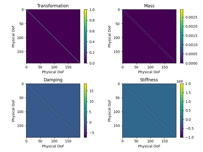
System matrices for the combined two beam system.
We can also verify by computing mode shapes or frequency responses. We can see that each mode shape generally consists of motion of only one structure, meaning the two systems are not connected.
combined_shapes = combined_system.eigensolution()
combined_geometry.plot_shape(combined_shapes)
Combined mode showing motion on just the first beam
Combined mode showing motion on just the second beam
We can also verify with frequency response functions. For example, we can compute a frequency response function between the end of one beam to the end of the other beam and verify that it is identically zero. We can first check to see the degrees of freedom of the beam.
combined_geometry.plot_coordinate(label_dofs=True)
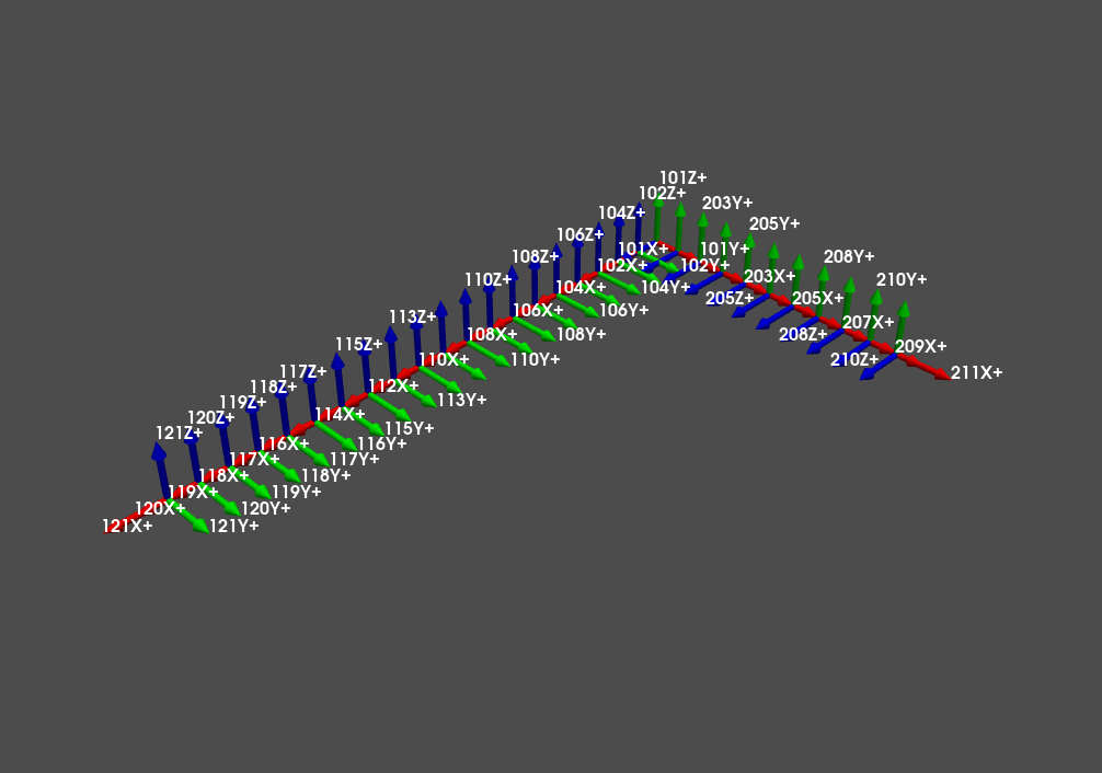
Degrees of freedom in the combined model
Then we can compute frequency response functions between the two structures and verify they are zero.
combined_frf = combined_system.frequency_response(
    frequency_lines,
    sdpy.coordinate_array(string_array='121Y+'),
    sdpy.coordinate_array(string_array='211Z+'))
In [68]: combined_frf.ordinate
Out[68]:
array([[[0.+0.j, 0.+0.j, 0.+0.j, 0.+0.j, 0.+0.j, 0.+0.j, 0.+0.j, 0.+0.j,
         ...
         0.+0.j, 0.+0.j, 0.+0.j, 0.+0.j, 0.+0.j, 0.+0.j, 0.+0.j, 0.+0.j]]])
Note in the coordinate plot that because we have rotated the beams, the degrees
of freedom do not necessarily match between the two systems. At the coincident
nodes, degree of freedom 101Z+ is not equivalent to 201Z+, but instead
it is equivalent 201Y+.
Applying Constraints to the System
In order to make the system behave as one structure instead of two separate
structures, we must apply constraints to the system. For example, we have
just identified that degrees of freedom 101Z+ and 201Y+ correspond
to the same position in space moving the same direction, so we should constrain
them to move together. We should apply similar constraints to the other
translations and rotations at that location. While SDynPy has the ability to
apply constraints directly to degrees of freedom in this way using the
substructure_by_coordinate
method of the System
object, it can also apply constraints automatically based on coincident geometry
using the
substructure_by_position
class method of the System.
This latter method will automatically determine which nodes are coincident,
as well as handle the different coordinate systems between the two systems.
constrained_system,constrained_geometry = sdpy.system.substructure_by_position(
    (damped_system,damped_system_2),
    (geometry,geometry_2))
If we compare our constrained system to the simply combined system, we will see that they have the same number of physical degrees of freedom, but the constrained system has six fewer internal degrees of freedom. These are lost due to the application of six constraints combining the rotational and translational degrees of freedom together. Each constraint removes one way the system can move.
In [69]: combined_system
Out[69]: System with 192 DoFs (192 internal DoFs)

In [70]: constrained_system
Out[70]: System with 192 DoFs (186 internal DoFs)
Now if we compute mode shapes or frequency response functions on this constrained system, we should see the two structures moving together. Additionally, if you apply a force to the first beam, the second beam will begin to move.
constrained_shapes = constrained_system.eigensolution()
constrained_geometry.plot_shape(constrained_shapes)

constrained_frf = constrained_system.frequency_response(
    frequency_lines,
    sdpy.coordinate_array(string_array='121Y+'),
    sdpy.coordinate_array(string_array='211Z+'))

constrained_frf.plot()
Constrained mode showing motion on both beams
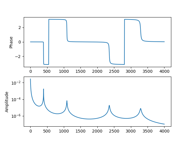
Frequency response function of the constrained system
For more advanced substructuring examples in SDynPy, see the example on the Transmission Simulator Method.
Frequency-Based Substructuring
In addition to assembling system matrices we can also perform substructuring in the frequency domain. We will need frequency response functions for all connection degrees of freedom, as well as the frequency response functions we wish to compute in the assembled system.
# Get the interface frfs
interface_dofs = sdpy.coordinate_array(
    [101,201],['X+','Y+','Z+','RX+','RY+','RZ+'],
    force_broadcast=True)

# Get the frfs that we want to compute in the constrained systems
response_dofs = sdpy.coordinate_array(string_array=['121Y+'])
reference_dofs = sdpy.coordinate_array(string_array=['211Z+'])

# Compute unconstrained frequency response functions
combined_frf = combined_system.frequency_response(
    frequency_lines,
    responses = np.concatenate((interface_dofs,response_dofs)),
    references = np.concatenate((interface_dofs,reference_dofs)))
To perform the substructuring, we will have to assemble the degree of freedom
pairs that we wish to constrain, similar to what we would have had to have done
had we used the
substructure_by_coordinate
method of the System
object instead of the
substructure_by_position
class method of the System. The
TransferFunctionArray
class also has a
substructure_by_coordinate
method that accepts degree of freedom pairs that will be used to apply
constraints.
dof_pairs = sdpy.coordinate_array(
    string_array = [['101Z+','201Y+'],
                    ['101Y+','201X+'],
                    ['101X+','201Z+'],
                    ['101RZ+','201RY+'],
                    ['101RY+','201RX+'],
                    ['101RX+','201RZ+']])

# Perform substructuring
constrained_frf_ss = combined_frf.substructure_by_coordinate(dof_pairs)
We can then compare frequency response functions across between the systems
to those computed from the combined system matrices to ensure they give the
same result. SDynPy’s book-keeping capabilities are useful here. We can index
the frequency response functions with a
CoordinateArray
object to pull out the desired function. We can get this
CoordinateArray
directly from the function against which we wish to compare, to ensure we are
comparing identical degrees of freedom. The
GUIPlot will allow easy comparisons
between functions.
# Get the coordinates
compare_coordinates = constrained_frf.coordinate

# Extract the correct functions by indexing with the coordinates
constrained_frf_compare = constrained_frf_ss[compare_coordinates]

# Plot the comparison
sdpy.GUIPlot(constrained_frf,constrained_frf_compare)
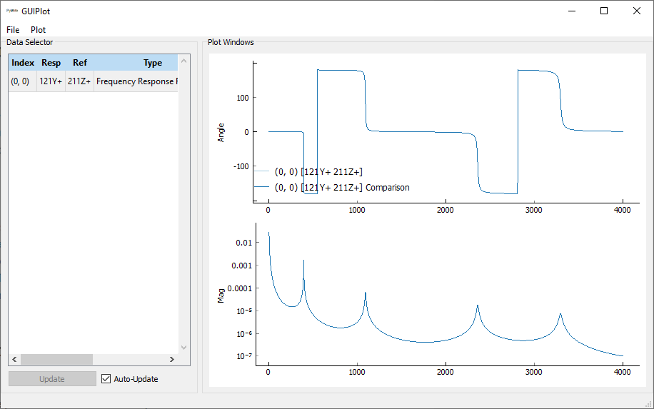
Frequency response comparison between the coupled system and frequency-based substructuring, showing identical results.
We can see that the results compare identically to the previous case of constraining the system matrices and then computing frequency response functions from the constrained system.