Data

Data is perhaps the most important aspect of Structural Dynamics. There are many different types of data that one may encounter in Structural Dynamics, from the simple time history tracking some quantity of interest over time, to more complex transfer functions, shock response spectra, or power spectral density matrices. Data objects in SDynPy can be viewed as somewhat of a “work in progress”, where commonly used data types such as time histories or transfer functions have a great deal of functionality defined for them, while less commonly used data types such as the correlation array have almost no specific functionality defined. Generally, functionality is added as it is required to be used, and with the main authors of SDynPy primarily working in vibration and modal analysis fields, users will find that types of data used in these fields are more fleshed out with functionality.

This document will demonstrate how data is defined and used in SDynPy. It will document basic operations that can be performed on data. Many SDynPy data objects also contain signal processing functionality; however, to reign in the scope of this document, signal processing operations will be discussed in later documentation.

Let’s import SDynPy and start looking at Data!

%gui qt
import sdynpy as sdpy
import numpy as np

SDynPy Data Objects

In order to provide commonality between all data objects in SDynPy while also providing the unique functionality that each data object requires, SDynPy users a inheritance-based model to define data objects. The parent class of all data classes in SDynPy is the NDDataArray object. As the name implies, this object inherits from and therefore has all of the functionality of the SdynpyArray and therefore a NumPy ndarray. SDynPy then defines subclasses of the NDDataArray to represent specific data types; for example the TimeHistoryArray represents data over time, the PowerSpectralDensityArray represents power spectral density functions, and the TransferFunctionArray represents transfer functions such as frequency response functions. Given the variety of types of data that can be represented by the NDDataArray and its subclasses, the sizes and types of the field are flexible. A time series represented by a TimeHistoryArray would generally consist of real data, whereas a frequency response function represented by a TransferFunctionArray would generally consist of complex data. Similarly a TimeHistoryArray may have a single degree of freedom (represented by a CoordinateArray) associated with each piece of data; however a TransferFunctionArray would generally have an input degree of freedom and an output degree of freedom associated with each piece of data. We will explore these differences throughout this document.

Similar to other SdynpyArray subclasses, the NDDataArray class and its subclasses have helper functions that aid in constructing of the objects. These generally will have the same name, except with snake_case capitalization instead of the CamelCase capitalization of the class. For example, a TimeHistoryArray object may be constructed with the time_history_array function. The exception to this rule is that there is not a specific helper function for the parent NDDataArray class, as this parent class will typically not be used directly.

Let’s start by creating a basic TimeHistoryArray object consisting of a sinusoidal signal.

num_sines = 10
frequencies = np.arange(num_sines)*10
timesteps = np.arange(1000)/1000
signal = np.sin(2*np.pi*frequencies[:,np.newaxis]*timesteps) # Will broadcast to a 10x1000 array
coordinate = sdpy.coordinate_array(1,'X+')

time_history = sdpy.time_history_array(
    abscissa = timesteps,
    ordinate = signal,
    coordinate = coordinate,
    comment1 = "A Comment",
    comment2 = "Another Comment",
    comment3 = "A Third Comment",
    comment4 = "A Fourth Comment",
    comment5 = "One Last Comment"
)

Note that when we create a NDDataArray object such as this TimeHistoryArray object, we must define at a minimum the abscissa, the ordinate, and the coordinate. The abscissa are the independent variables; for a time history, this would be the value of time at each sample. For a spectral quantity such as a frequency response function or a power spectral density function, this would be the frequency lines. The ordinate field is then the dependent variable. In the case of a time history, this would be the value of the function at each time step. Note that when defining abscissa and ordinate, SDynPy does not handle units. Users should ensure their data is in a consistent unit systems, because no conversions will be done by SDynPy.

Users must also assign degree of freedom information to each item in the NDDataArray using the coordinate argument. These will be the standard SDynPy CoordinateArray objects discussed previously i`Coordinates`_.

Finally, users can assign up to five comments for each item in the array. These could be used to store any information pertinent to the analysis. Units (g, m, m/s, N, etc.) or unit type (force, acceleration, etc.) may be valid information to store, but it is worth mentioning again: SDynPy will not attempt to parse these comments when doing any analysis on the data, and will not try to perform unit conversions for the user.

Now that we have a NDDataArray subclass defined, let’s look at some of its fields and dtype.

time_history.fields

('abscissa',
 'ordinate',
 'comment1',
 'comment2',
 'comment3',
 'comment4',
 'comment5',
 'coordinate')

time_history.dtype

dtype([('abscissa', '<f8', (1000,)), ('ordinate', '<f8', (1000,)), ('comment1', '<U80'), ('comment2', '<U80'), ('comment3', '<U80'), ('comment4', '<U80'), ('comment5', '<U80'), ('coordinate', [('node', '<u8'), ('direction', 'i1')], (1,))])

We can see the for each function in the TimeHistoryArray, we have floating point fields abscissa and ordinate. We can see that these fields have shape (1000,), which represents the 1000 time steps in our sine wave.

We also see the five comment fields, comment1 through comment5, which are strings. The choice for five comment fields stems from the Universal File Format Dataset 58, which is used to store functions at nodal degrees of freedom. Dataset 58 stores five ID Line records, and SDynPy objects typically try to match the corresponding Universal File Format object.

The last field is the coordinate field, and we note that this field has shape (1,). This means for that this object, there is one coordinate for each entry in the array. We also see that the coordinate field is a compound dtype, which contains node and direction fields. Readers having read the Coordinates will recognize this as the dtype of the CoordinateArray object, meaning NDDataArray objects store coordinate information as a CoordinateArray.

time_history.dtype['coordinate']

dtype(([('node', '<u8'), ('direction', 'i1')], (1,)))

# Create a dummy coordinate array so we can see its dtype
sdpy.coordinate_array(1,1).dtype

dtype([('node', '<u8'), ('direction', 'i1')])

Indeed, if we request the coordinate field of a NDDataArray object, we will receive a CoordinateArray object.

time_history.coordinate

coordinate_array(string_array=
array([['1X+'],
       ['1X+'],
       ['1X+'],
       ['1X+'],
       ['1X+'],
       ['1X+'],
       ['1X+'],
       ['1X+'],
       ['1X+'],
       ['1X+']], dtype='<U3'))

For comparison, let’s create a TransferFunctionArray object and compare its dtype.

freqs = np.arange(1000)
ordinate = np.random.randn(1000)
coordinate = sdpy.coordinate_array([1,2],'X+') # Uses broadcasting
tf = sdpy.transfer_function_array(
    abscissa = freqs,
    ordinate = ordinate,
    coordinate = coordinate
)

tf.dtype

dtype([('abscissa', '<f8', (1000,)), ('ordinate', '<c16', (1000,)), ('comment1', '<U80'), ('comment2', '<U80'), ('comment3', '<U80'), ('comment4', '<U80'), ('comment5', '<U80'), ('coordinate', [('node', '<u8'), ('direction', 'i1')], (2,))])

We see that for this TransferFuntionArray, the ordinate field is now a complex number <c16 compared to a real number <f8 like in the TimeHistoryArray. Similarly, the shape of the coordinate dtype is now (2,) instead of (1,), meaning there are two coordinates for each of the transfer functions.

Recall from previous documentation that when a dtype has a shape associated with it, that shape will be appended to the end of the shape of the array itself. For example, our sine time history currently has shape (10,)

time_history.shape

(10,)

If we then look at the coordinate field, which has dtype with shape (1,), we should see its shape be (10,1).

time_history.coordinate.shape

(10, 1)

This can be a point of confusion when working with NDDataArray subclasses, particularly with the subclasses that have coordinate fields with shape (1,). Many users will forget to include this last dimension on the coordinate field. This is particularly detrimental because NumPy will not broadcast the incorrect shape of (10,) to the correct shape of (10,1). Per NumPy broadcasting rules, the (1,) dimension will be expanded to match the provided dimension, so the final shape will instead be (10,10), which will not be correct.

Similarly, we see that the abscissa and ordinate fields also have non-scalar dtype shapes of (1000,). This means that these fields will have a shape of (10,1000).

time_history.ordinate.shape

(10, 1000)

Creating Data from Scratch

Now that we have discusssed a bit about the NDDataArray object and its subclasses, let’s look more closely at how we can construct one. We will assume we have time history that are sines and cosines, and use that to create our data arrays. Here we will pay more attention to the sizes of the arrays to demonstrate exactly how the functions work.

First, we will construct a multidimensional array of data that we will use for the ordinate. We will try to end up with a 5 x 2 array of time histories, where each row corresponds to an increasing frequency, and the two columns correspond to sines and cosines (or 0 and 90 degree phases, respectively). We will create 1000 time steps for each function from 0 to 1 (or rather, slightly less than 1 due to Python’s open interval).

# We will use broadcasting to help us construct these arrays.
frequencies = ((np.arange(5)+1)*10)[:,np.newaxis,np.newaxis] # Frequency is the first dimension
phases = (np.arange(2)*np.pi/2)[:,np.newaxis] # Phase is the second dimension
timesteps = np.arange(1000)/1000 # Timestep is the last dimension.
signal_ordinate = np.sin(2*np.pi*frequencies*timesteps+phases) # 3D broadcasting occuring in this last function.

# Check the shape
signal_ordinate.shape

(5, 2, 1000)

We can see we have our 5 x 2 sine waves each with 1000 time steps. When we construct a TimeHistoryArray using the time_history_array function with this value as the ordinate argument, the time_history_array function will peel off the last dimension (1000) to use as the shape of the ordinate dtype, and the remaining dimensions (5 x 2) will be used as the shape of the TimeHistoryArray itself.

We could also create a variable with shape (5,2,1000) to use as the abscissa argument. However the helper functions generally use broadcasting across the arguments, so our current timesteps variable with shape (1000) will automatically be broadcast to the correct (5,2,1000) shape. We do, however, need to construct the entry for the coordinate argument. Recalling what we learned previously, we know that a TimeHistoryArray will have a coordinate field with dtype that has the shape of (1,), meaning there is one degree of freedom per function. Knowing that our TimeHistoryArray will have shape (5,2), we should append the dtype shape to this value to get the necessary shape for our CoordinateArray, which is (5,2,1). We can do this by creating a shape (5,2) CoordinateArray then using np.newaxis to add the last dimension.

coordinates = sdpy.coordinate_array( # Use broadcasting to get 5x2
    np.arange(5)[:,np.newaxis]+1,    # Nodes have shape 5x1
    ['X+','Y+']                      # Directions have shape 2
    )[...,np.newaxis]                # Add the newaxis at the end

# Check the size
coordinates.shape

(5, 2, 1)

Now we can pass this information to the time_history_array function to construct our TimeHistoryArray object.

time_histories = sdpy.time_history_array(
    abscissa = timesteps,
    ordinate = signal_ordinate,
    coordinate = coordinates
)

If we want to know more about our data, we can simply type its name into the terminal.

time_histories

TimeHistoryArray with shape 5 x 2 and 1000 elements per function

Here it tells us the shape of our TimeHistoryArray object as well as how many timesteps are in it.

As a second example with a different shape, let’s compute some transfer functions. There will be some slight differences between this and the previous example: the ordinate field can be complex for a TransferFunctionArray and the coordinate field will now have dtype with shape (2,). Another difference is that the abscissa value is now frequency lines instead of time steps; however since SDynPy does not handle units, it will not know the difference if we pass our timesteps array from the previous example as the abscissa for the present example.

Let’s start by producing a complex where we compute the sine of the arguments the real part and the cosine of the argument as the imaginary part.

# We will use broadcasting to help us construct these arrays.
frequencies = ((np.arange(5)+1)*10)[:,np.newaxis,np.newaxis] # Frequency is the first dimension
phases = (np.arange(2)*np.pi/2)[:,np.newaxis] # Phase is the second dimension
timesteps = np.arange(1000)/1000 # Timestep is the last dimension.
signal_ordinate = np.sin(2*np.pi*frequencies*timesteps+phases) + 1j*np.cos(2*np.pi*frequencies*timesteps+phases) # 3D broadcasting occuring in this last function.

# Check the shape
signal_ordinate.shape

(5, 2, 1000)

We will also need to compute a coordinate field with size (5,2,2) where the last 2 is due to the shape of the coordinate field’s dtype. Here we will not use np.newaxis because the new axis we need must have length 2 instead of length 1. We will instead rely entirely on broadcasting.

coordinates = sdpy.coordinate_array(            # Use broadcasting to get 5x2x2
    np.arange(5)[:,np.newaxis,np.newaxis]+1,    # Nodes have shape 5x1x1
    [['X+','Z+'],
     ['Y+','Z+']]                               # Directions have shape 2 x 2
    )

# Check the size
coordinates.shape

(5, 2, 2)

Let’s then create the TransferFunctionArray using the helper function transfer_function_array.

tfs = sdpy.transfer_function_array(
    abscissa = timesteps,
    ordinate = signal_ordinate,
    coordinate = coordinates
)

Again, we can type the name into the terminal to get more information.

tfs

TransferFunctionArray with shape 5 x 2 and 1000 elements per function

Visualizing Data

Up to this point, we have simply trusted SDynPy that it created our data correctly. However, we would often like to verify this is the case by visualizing the data. All NDDataArray subclasses have a plot method. Some subsclasses override the parent class method to add their own functionality. Let’s start with the TimeHistoryArray object.

time_histories.plot()

<Axes: >

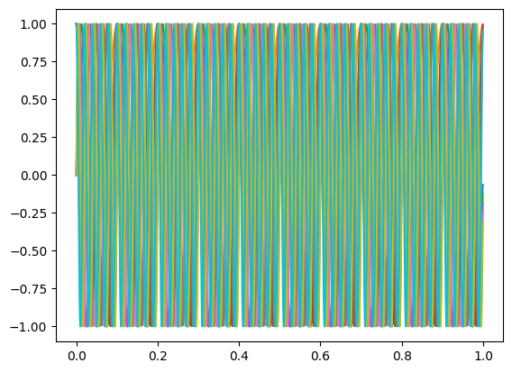
We can see by simply calling the plot method, it has plotted all of the time histories on a single figure. This may or may not be desirable. If many functions are plotted, the plots may get busy and hard to read. The one_axis argument of the function, which defaults to True can be set to False to plot all figures on separate plots.

time_histories.plot(one_axis=False)

array([[<Axes: ylabel='1X+'>, <Axes: ylabel='1Y+'>, <Axes: ylabel='2X+'>],
       [<Axes: ylabel='2Y+'>, <Axes: ylabel='3X+'>, <Axes: ylabel='3Y+'>],
       [<Axes: ylabel='4X+'>, <Axes: ylabel='4Y+'>, <Axes: ylabel='5X+'>],
       [<Axes: ylabel='5Y+'>, <Axes: >, <Axes: >]], dtype=object)

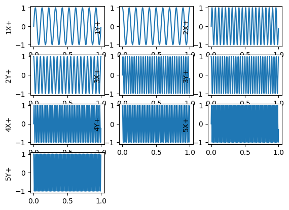
This may also produce varying levels of success depending on how many plots are plotted on the figure. Note in the above, the axis labels overlay the adjacent plots. To accomodate this, the plot method also takes optional arguments to allow us to customize the result and make it look more appealing. These arguments are generally keyword arguments to the lower level Matplotlib function calls.

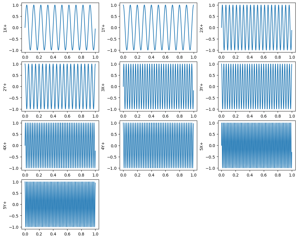
time_histories.plot(one_axis=False,subplots_kwargs={'layout':'constrained','figsize':(10,8)})

array([[<Axes: ylabel='1X+'>, <Axes: ylabel='1Y+'>, <Axes: ylabel='2X+'>],
       [<Axes: ylabel='2Y+'>, <Axes: ylabel='3X+'>, <Axes: ylabel='3Y+'>],
       [<Axes: ylabel='4X+'>, <Axes: ylabel='4Y+'>, <Axes: ylabel='5X+'>],
       [<Axes: ylabel='5Y+'>, <Axes: >, <Axes: >]], dtype=object)

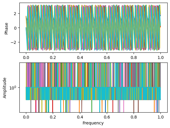
For certain types of data, the plot method is overridden to provide more appropriate functionality. For example, our TransferFunctionArray is a complex number. If we simply plot it, we will see magnitude and phase. Note that since we build our functions with the real part as a sine and the complex part as the cosine, the magnitude will be identically 1 while the phase changes with frequency.

tfs.plot()

array([<Axes: ylabel='Phase'>,
       <Axes: xlabel='Frequency', ylabel='Amplitude'>], dtype=object)

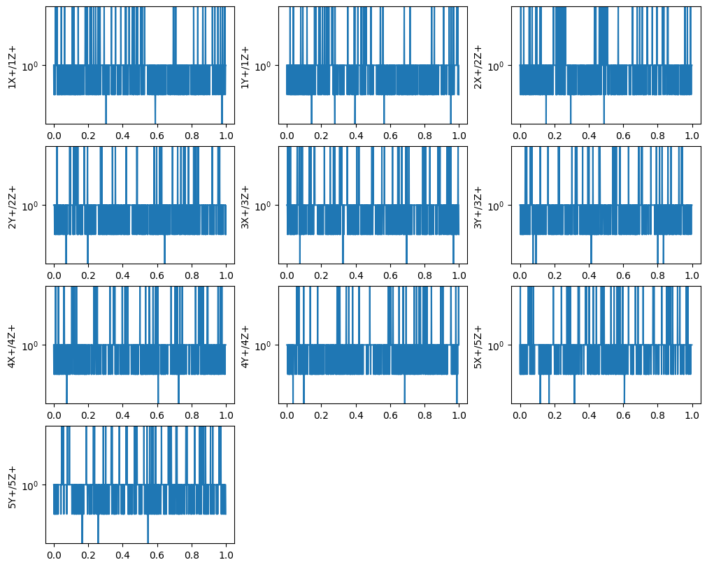
If we plot on multiple axes, we can see that it will by default plot the magnitude of the transfer function.

tfs.plot(one_axis=False,subplots_kwargs={'layout':'constrained','figsize':(10,8)})

array([[<Axes: ylabel='1X+/1Z+'>, <Axes: ylabel='1Y+/1Z+'>,
        <Axes: ylabel='2X+/2Z+'>],
       [<Axes: ylabel='2Y+/2Z+'>, <Axes: ylabel='3X+/3Z+'>,
        <Axes: ylabel='3Y+/3Z+'>],
       [<Axes: ylabel='4X+/4Z+'>, <Axes: ylabel='4Y+/4Z+'>,
        <Axes: ylabel='5X+/5Z+'>],
       [<Axes: ylabel='5Y+/5Z+'>, <Axes: >, <Axes: >]], dtype=object)

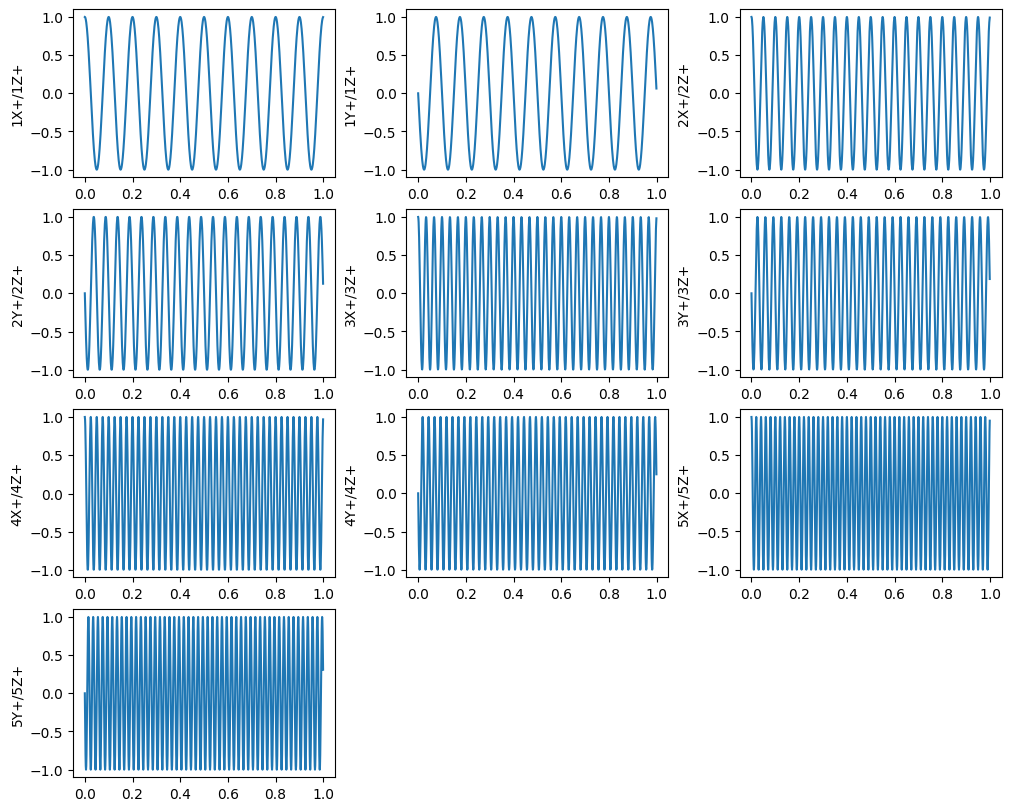
However, we can specify which part of the TransferFunctionArray to plot using the part argument.

tfs.plot(one_axis=False,subplots_kwargs={'layout':'constrained','figsize':(10,8)},part='imag')

array([[<Axes: ylabel='1X+/1Z+'>, <Axes: ylabel='1Y+/1Z+'>,
        <Axes: ylabel='2X+/2Z+'>],
       [<Axes: ylabel='2Y+/2Z+'>, <Axes: ylabel='3X+/3Z+'>,
        <Axes: ylabel='3Y+/3Z+'>],
       [<Axes: ylabel='4X+/4Z+'>, <Axes: ylabel='4Y+/4Z+'>,
        <Axes: ylabel='5X+/5Z+'>],
       [<Axes: ylabel='5Y+/5Z+'>, <Axes: >, <Axes: >]], dtype=object)

While the typical plot method allows you easily visualize moderately-sized datasets, as datasets grow larger, it can be difficult to put all of the data on one screen at once. In this case, it might be easier to interactively explore the data. SDynPy’s GUIPlot capability will bring up a graphical user interface window in which the user will be presented with all of the functions that are available. The user can then click on one or more of these functions to visualize. To quickly bring up a GUIPlot window, users can call the gui_plot method.

Within this window, users can select the functions to plot from the table on the left. The line width of the plots and sizes of markers (if used) can be adjusted. The plot window on the right can be interactively zoomed to visualize certain portions of the plot.

time_histories.gui_plot()

<sdynpy.core.sdynpy_data.GUIPlot at 0x1882133f2f0>

For more functionality, including the ability to compare different datasets, the GUIPlot class can be called directly. Different datasets can be passed in as arguments or keyword arguments (in the latter case, the keyword labels will be used as the legend entries). Additionally markers at specific times can be plotted with different styles. See the documentation of GUIPlot for the full range of capabilities.

sdpy.GUIPlot(Sines = time_histories[:,0],Cosines = time_histories[:,1],
             abscissa_markers = [0,0.25,0.5],
             abscissa_marker_labels = ['0','1/4','1/2'],
             abscissa_marker_type = 'vline')

Warning: Coordinates not consistent for dataset Cosines

<sdynpy.core.sdynpy_data.GUIPlot at 0x1882133f6e0>

For complex data types, the GUIPlot can change how the complex values are presented (real/imaginary/magnitude/phase). As well as whether or not the plot should use logarithmic scaling on each axis.

tfs.gui_plot()

<sdynpy.core.sdynpy_data.GUIPlot at 0x18821b5f0b0>

Indexing NDDataArrays

In Structural Dynamics, we often would like to select specific pieces of data on which operations will be performed. Because NDDataArray objects are NumPy arrays, indexing is performed the same way on both NDDataArray objects and NumPy arrays.

time_histories

TimeHistoryArray with shape 5 x 2 and 1000 elements per function

time_histories[2,1]

TimeHistoryArray with shape  and 1000 elements per function

time_histories[0,:]

TimeHistoryArray with shape 2 and 1000 elements per function

time_histories[[0,3,4],[0,1,0]]

TimeHistoryArray with shape 3 and 1000 elements per function

While standard NumPy indexing can be used successfully, it can be error-prone. Often, one is looking for a specific degree of freedom, and using NumPy indexing, one must first find the index corresponding to that degree of freedom.

# Define the coordinate we are looking for
desired_dof = sdpy.coordinate_array(1,'X+')

# Recall coordinate field is ... x 1, so this is why we do all across
# the last axis.
dof_matches = np.all(time_histories.coordinate == desired_dof,axis=-1)

print('Matching Coordinates:')
print(dof_matches)

# Select the time history with that coordinate
matching_time_history = time_histories[dof_matches]

print('\nFound Time History: ')
print(matching_time_history)
print('With Coordinate:')
print(matching_time_history.coordinate)

Matching Coordinates:
[[ True False]
 [False False]
 [False False]
 [False False]
 [False False]]

Found Time History:
TimeHistoryArray with shape 1 and 1000 elements per function
With Coordinate:
[['1X+']]

This is passable; however it is many lines of code for a single operation. Additionally, it does not generalize well to more interesting circumstances. For example, what if we wanted to find the time history associated with the 1X- direction?

# Define the coordinate we are looking for
desired_dof = sdpy.coordinate_array(1,'X-')

# Recall coordinate field is ... x 1, so this is why we do all across
# the last axis.
dof_matches = np.all(time_histories.coordinate == desired_dof,axis=-1)

print('Matching Coordinates:')
print(dof_matches)

# Select the time history with that coordinate
matching_time_history = time_histories[dof_matches]

print('\nFound Time History: ')
print(matching_time_history)
print('With Coordinate:')
print(matching_time_history.coordinate)

Matching Coordinates:
[[False False]
 [False False]
 [False False]
 [False False]
 [False False]]

Found Time History:
TimeHistoryArray with shape 0 and 1000 elements per function
With Coordinate:
[]

We now get no matches, even though we should be able to match the same function but just flip the sign on the function. To handle this common occurrance in a more user-friendly way, SDynPy allows users to index NDDataArray objects directly with a CoordinateArray object. SDynPy will then select the functions that match the coordinates for each coordinate. This will accomodate sign flips and multidimensionality as well.

One important point to remember is that the shape of the coordinate field of the NDDataArray must be respected. This means when selecting for TimeHistoryArray objects, the CoordinateArray should have shape (...,1) or for TransferFunctionArray objects, the CoordinateArray should have shape (...,2), where then ... will be the shape of the output NDDataArray.

# This has shape (3,))
desired_dofs = sdpy.coordinate_array([1,3,4],'X+')

# If we don't make it (3,1), the indexing operation will fail
time_histories[desired_dofs]

---------------------------------------------------------------------------
IndexError                                Traceback (most recent call last)
File ~\Documents\Local_Repositories\sdynpy\src\sdynpy\core\sdynpy_data.py:981, in NDDataArray.__getitem__(self, key)
    980 try:
--> 981     index_array[index] = np.where(
    982         np.all(positive_coordinates == positive_key, axis=-1))[0][0]
    983 except IndexError:

IndexError: index 0 is out of bounds for axis 0 with size 0

During handling of the above exception, another exception occurred:

ValueError                                Traceback (most recent call last)
Cell In[35], line 5
      2 desired_dofs = sdpy.coordinate_array([1,3,4],'X+')
      4 # If we don't make it (3,1), the indexing operation will fail
----> 5 time_histories[desired_dofs]

File ~\Documents\Local_Repositories\sdynpy\src\sdynpy\core\sdynpy_data.py:984, in NDDataArray.__getitem__(self, key)
    981         index_array[index] = np.where(
    982             np.all(positive_coordinates == positive_key, axis=-1))[0][0]
    983     except IndexError:
--> 984         raise ValueError('Coordinate {:} not found in data array'.format(str(key[index])))
    985 return_shape = flat_self[index_array].copy()
    986 if self.function_type in [FunctionTypes.COHERENCE, FunctionTypes.MULTIPLE_COHERENCE]:

ValueError: Coordinate ['1X+' '3X+' '4X+'] not found in data array

# If we make it (3,1), then it will succeed
desired_dofs = desired_dofs[:,np.newaxis]
time_histories[desired_dofs].coordinate

coordinate_array(string_array=
array([['1X+'],
       ['3X+'],
       ['4X+']], dtype='<U3'))

As stated previously, this operation handles multidimensionality and sign flipping. Let’s set up an indexing operation that will pull the desired degrees of freedom while also exercising multidimensionality and sign flipping.

desired_dofs = sdpy.coordinate_array(
    [[3],[1],[4]], # 3x1
    ['X+','X-'],   # 1x2 (implicitly)
)[...,np.newaxis]  # add newaxis for 3x2x1

# We should get a 3x2 array, where the second column
# is the first column with the sign flipped.
desired_time_histories = time_histories[desired_dofs]

print(desired_time_histories)
print(desired_time_histories.coordinate)

TimeHistoryArray with shape 3 x 2 and 1000 elements per function
[[['3X+']
  ['3X-']]

 [['1X+']
  ['1X-']]

 [['4X+']
  ['4X-']]]

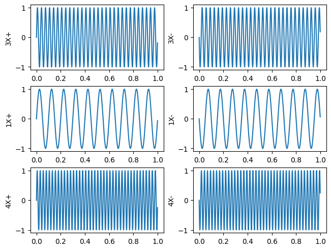
If we plot the functions, we should see that the different sign on the coordinate automatically flips the sign on the data as well. We can also see that we have received the data in the same order as we requested it. This enables very powerful indexing operations to be performed with minimal chance for bookkeeping errors.

desired_time_histories.plot(one_axis=False,subplots_kwargs={'layout':'constrained'})

array([[<Axes: ylabel='3X+'>, <Axes: ylabel='3X-'>],
       [<Axes: ylabel='1X+'>, <Axes: ylabel='1X-'>],
       [<Axes: ylabel='4X+'>, <Axes: ylabel='4X-'>]], dtype=object)

Reading and Writing to NumPy Files

SDynPy does not have a native storage format for its data types. However, being built mostly on NumPy arrays, it is almost trivial to use NumPy format for storage. A NDDataArray object can be saved using its NDDataArray.save method. It will be written to a NumPy .npz file containing the equivalent NumPy structured array. One additional field will be saved in the .npz file, which is subclass of the array. Since the fields of each NDDataArray are identical across types, the subclass of the NDDataArray could not be reconstructed from the field names alone. Therefore, SDynPy must save this property in order to load it back in correctly.

time_histories.save('time_histories.npz')

To load a NDDataArray object from the file, one can simply call the class method NDDataArray.load or its alias data.load, which will recognize the subclass within the file and correctly reconstruct the object.

# Class method
time_histories_from_npz = sdpy.NDDataArray.load('time_histories.npz')
# Equivalent module-level alias
time_histories_from_npz = sdpy.data.load('time_histories.npz')

Writing to Matlab Files

Many structural dynamicists utilize the Matlab programming language to perform structural dynamics analysis. Therefore, it is useful to be able to share data between SDynPy and Matlab. SDynPy can save data in a NDDataArray to a .mat file using the savemat method.

time_histories.savemat('time_histories.mat')

The .mat file will contain fields with the same names and shapes as the NDDataArray object. The coordinate field will be saved a a structure with node and direction fields.

from scipy.io import loadmat
time_history_matlab_data = loadmat('time_histories.mat')

time_history_matlab_data.keys()

dict_keys(['__header__', '__version__', '__globals__', 'abscissa', 'ordinate', 'comment1', 'comment2', 'comment3', 'comment4', 'comment5', 'coordinate'])

Because a .mat file can have any format, there is no dedicated loadmat equivalent to savemat. Since .mat files may have any field names, it is up to the user to open up the .mat file using their tool of choice, parse out the data required to construct a NDDataArray object, and create the object manually from the underlying data.

Summary

In summary, the NDDataArray object in SDynPy is used to store data information. Many different types of data can be represented in SDynPy, and each of these is represented as a subclass of NDDataArray.

The NDDataArray objects store independent and dependent variables in abscissa and ordinate fields. The degree of freedom information is stored simultaneously in a CoordinateArray object that is the shape of the NDDataArray with the shape of the coordinate field itself appended. This is because different types of data might be associated with different numbers of degrees of freedom. A time history, for example, will have one degree of freedom associated with it. A frequency response function, however, will have an input and an output degree of freedom associated with each function.

NDDataArray objects (or its subclasses) can be plotted easily with the plot method, which also accepts numerous arguments to customize the generated figure. However, if many functions are to be plotted, it may be easier to interactively interrogate the data with GUIPlot. GUIPlot is well suited to compare data and apply annotations as well.

NDDataArray objects (or its subclasses) can be indexed using standard NumPy indexing operations. However, they can also be indexed using CoordinateArray objects. These objects can be multidimensional or contain direction flips compared to the underlying data. SDynPy will gracefully return the item corresponding to the requested CoordinateArray in the shape and order requested with any sign flips applied.

NDDataArray objects (or its subclasses) can be saved and loaded to disk in NumPy format as .npz files. It is also straightforward to write the data to a Matlab .mat file.

This document has only scratched the surface of the functionality available in the NDDataArray class and its subclasses. A large number of signal processing methods are available. These methods will require full knowledge of SDynPy’s core capabilities, and will be addressed in subsequent documentation.