System
In structural dynamics, we often work with dynamic systems that represent real or simulated dynamic objects. The dynamic system originates from the second-order differential equations of motion for a structure.
The system displayed above consists of mass, damping, and system matrices (\(\mathbf{M}\), \(\mathbf{C}\), and \(\mathbf{K}\), respectively) that determine how the degrees of freedom of the system (\(\mathbf{x}\)) change over time due to some input (\(\mathbf{F}\)). This equation might represent a physical system where responses \(\mathbf{x}\) and inputs \(\mathbf{F}\) correspond to physical displacements and forces.
However, in general, we may also have the equations of motion representing a reduced or transformed system. For example, in the case of modal analysis, we may represent the equations of motion as the response of the modes of the structure. If the mode shape matrix is represented as \(\mathbf{\Phi}\) and the modal degrees of freedom \(\mathbf{q}\) where \(\mathbf{x} = \mathbf{\Phi}\mathbf{q}\), then the equations of motion can be written as
or
where \(\mathbf{x} = \mathbf{\Phi}\mathbf{q}\) and \(\tilde{f} = \mathbf{\Phi}^T\mathbf{F}\). This represents a system that has been transformed from a physical system to a reduced system through the transformation matrix \(\mathbf{\Phi}\). The physical forces \(\mathbf{F}\) are transformed to modal forces \(\tilde{\mathbf{f}}\) using the transformation matrix, which are applied to the reduced system, and the reduced responses \(\mathbf{q}\) are then expanded back to physical responses \(\mathbf{x}\) again with that transformation matrix. We can also see that the physical system is simply a specific case of the general reduced equation where the transformation matrix is the identity matrix.
To represent dynamic systems, SDynPy uses the general reduced form of these systems of equations. This allows SDynPy to describe the system and any transformation applied to it. SDynPy will also track the coordinates associated with each entry in the input and response vectors, allowing bookkeeping to be automated.
This document will demonstrate how Systems are defined and used in SDynPy. We will start by defining the System object, then walk through different use-cases in SDynPy.
Let’s import SDynPy and start looking at Systems!
[1]:
import sdynpy as sdpy
import numpy as np
import matplotlib.pyplot as plt
SDynPy System Objects
In SDynPy, the object used to represent dynamic systems is the System. Unlike the documentation covered so far, System objects are not NumPy arrays. Similar to Geometry objects, we do not typically store arrays of systems, and if we do, the typical Python data structures such as lists or dictionaries are typically sufficient.
SDynPy system objects will store mass, damping, and stiffness matrices, as well as the coordinates associated with each degree of freedom in these matrices. The System object may also store a general transformation matrix that will be used as the input and output transformation from the reduced space, if appropriate. If a physical system is represented, this transformation will be the identity matrix.
Creating a System from Scratch
When defining a system, we typically have some structure we are trying to model. Somehow we must compute mass, stiffness, and damping matrices for this structure. For a spring-mass-damper model, these matrices can often be constructed by hand using the discrete elements in the model. For a finite element model, the mass, stiffness, and damping might need to come from external software and be imported into SDynPy. For a reduced system, the mass, stiffness, damping, and transformation values may be known from some other analysis (for example, a modal system might have the identity matrix as its mass matrix, diagonal stiffness and damping based on the natural frequency and damping ratio, and the transformation would be the mode shape matrix). Once these matrices are known, we can combine them with a CoordinateArray representing the degree of freedom for each row and column of the matrices to construct the final System object.
For this example, we will assume the form of the system as a series of masses connected by springs.
[2]:
ndofs = 10

# Connections will be 2 on the diagonal and -1 on the off-diagonal
connectivity_matrix = np.eye(ndofs) # Diagonal, we will double this when we add the transpose
connectivity_matrix[np.arange(ndofs-1),np.arange(ndofs-1)+1] = -1 # Off-diagonal
connectivity_matrix = connectivity_matrix + connectivity_matrix.T # Make symmetric
connectivity_matrix[-1,-1] = 1 # Make the end free instead of fixed.

mass = np.eye(ndofs)
stiffness = connectivity_matrix*1e6
damping = connectivity_matrix*1e2
For this system, we will assume that the transformation is identity, so we will not define it. We will assign coordinates for each of the degrees of freedom as increasing node numbers in the X+ direction.
[3]:
coordinates = sdpy.coordinate_array(np.arange(ndofs)+1,'X+')
Now we have enough information to construct a System object.
[4]:
system = sdpy.System(
    coordinates,
    mass,
    stiffness,
    damping,
)
By typing in the name into the terminal, we can get more information about the system.
[5]:
system
[5]:
System with 10 DoFs (10 internal DoFs)
We note that SDynPy is reporting both 10 degrees of freedom and 10 internal (state) degrees of freedom, meaning the system is not reduced at all.
We can access the internal matrices though the mass, stiffness, or damping properties, or their associated aliases, M, K, or C.
[6]:
system.damping
[6]:
array([[ 200., -100.,    0.,    0.,    0.,    0.,    0.,    0.,    0.,
           0.],
       [-100.,  200., -100.,    0.,    0.,    0.,    0.,    0.,    0.,
           0.],
       [   0., -100.,  200., -100.,    0.,    0.,    0.,    0.,    0.,
           0.],
       [   0.,    0., -100.,  200., -100.,    0.,    0.,    0.,    0.,
           0.],
       [   0.,    0.,    0., -100.,  200., -100.,    0.,    0.,    0.,
           0.],
       [   0.,    0.,    0.,    0., -100.,  200., -100.,    0.,    0.,
           0.],
       [   0.,    0.,    0.,    0.,    0., -100.,  200., -100.,    0.,
           0.],
       [   0.,    0.,    0.,    0.,    0.,    0., -100.,  200., -100.,
           0.],
       [   0.,    0.,    0.,    0.,    0.,    0.,    0., -100.,  200.,
        -100.],
       [   0.,    0.,    0.,    0.,    0.,    0.,    0.,    0., -100.,
         100.]])
[7]:
system.C
[7]:
array([[ 200., -100.,    0.,    0.,    0.,    0.,    0.,    0.,    0.,
           0.],
       [-100.,  200., -100.,    0.,    0.,    0.,    0.,    0.,    0.,
           0.],
       [   0., -100.,  200., -100.,    0.,    0.,    0.,    0.,    0.,
           0.],
       [   0.,    0., -100.,  200., -100.,    0.,    0.,    0.,    0.,
           0.],
       [   0.,    0.,    0., -100.,  200., -100.,    0.,    0.,    0.,
           0.],
       [   0.,    0.,    0.,    0., -100.,  200., -100.,    0.,    0.,
           0.],
       [   0.,    0.,    0.,    0.,    0., -100.,  200., -100.,    0.,
           0.],
       [   0.,    0.,    0.,    0.,    0.,    0., -100.,  200., -100.,
           0.],
       [   0.,    0.,    0.,    0.,    0.,    0.,    0., -100.,  200.,
        -100.],
       [   0.,    0.,    0.,    0.,    0.,    0.,    0.,    0., -100.,
         100.]])
Note that since we did not specify a transformation, the transformation is the identity matrix.
[8]:
system.transformation
[8]:
array([[1., 0., 0., 0., 0., 0., 0., 0., 0., 0.],
       [0., 1., 0., 0., 0., 0., 0., 0., 0., 0.],
       [0., 0., 1., 0., 0., 0., 0., 0., 0., 0.],
       [0., 0., 0., 1., 0., 0., 0., 0., 0., 0.],
       [0., 0., 0., 0., 1., 0., 0., 0., 0., 0.],
       [0., 0., 0., 0., 0., 1., 0., 0., 0., 0.],
       [0., 0., 0., 0., 0., 0., 1., 0., 0., 0.],
       [0., 0., 0., 0., 0., 0., 0., 1., 0., 0.],
       [0., 0., 0., 0., 0., 0., 0., 0., 1., 0.],
       [0., 0., 0., 0., 0., 0., 0., 0., 0., 1.]])
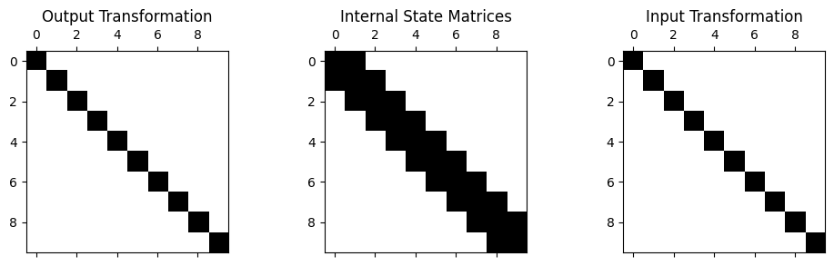
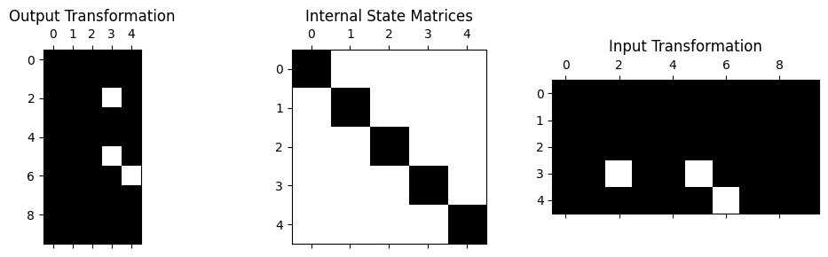
We can visualize the connectivity of the system (which degrees of freedom are attached to each other) using the spy method. This will produce a visualization of the internal state matrices as well as the transformations.
[9]:
system.spy()
[9]:
array([<Axes: title={'center': 'Output Transformation'}>,
       <Axes: title={'center': 'Internal State Matrices'}>,
       <Axes: title={'center': 'Input Transformation'}>], dtype=object)
Simulating the System
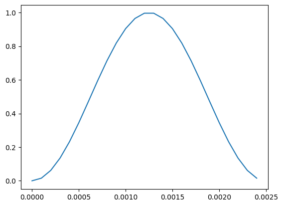
Once we have a system object, we may wish to see how it would respond if we applied a forces to specific degrees of freedom. Let’s apply a shock-like force at the middle of the structure and a second force 1/4 of the way up the structure. We will then integrate equations of motion to recover the response. To do this, we simply need to construct the forces as a TimeHistoryArray with the correct degrees of freedom, and pass it to the time_integrate method.
[10]:
time_step = 1e-4 # Seconds
pulse = np.sin(400*np.pi*np.arange(25)*time_step)**2

fig,ax = plt.subplots()
ax.plot(np.arange(pulse.size)*time_step,pulse)
[10]:
[<matplotlib.lines.Line2D at 0x22a65d3d1d0>]
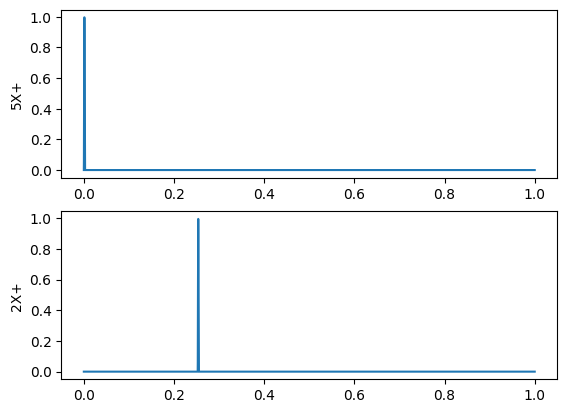
[11]:
# Set up the full ordinate
signal_time = 1 # Seconds
signal = np.zeros((2,int(signal_time/time_step)))
signal[0,:25] = pulse # First hit
signal[1,2525:2550] = pulse # Second hit sometime later

# Set up the coordinate
force_locations = sdpy.coordinate_array(
    [
        ndofs//2, # Halfway on the part
        ndofs//4, # 1/4 of the way on the part
    ],
    'X+'
)[:,np.newaxis] # Remember to make it shape (2,1) instead of shape 2

# Create the time history array
forces = sdpy.time_history_array(
    abscissa = np.arange(signal.shape[-1])*time_step,
    ordinate = signal,
    coordinate = force_locations
)

forces.plot(one_axis=False)
[11]:
array([<Axes: ylabel='5X+'>, <Axes: ylabel='2X+'>], dtype=object)
Now we can apply these forces to the System object using time_integrate. Optional arguments to this function can allow us to specify which degrees of freedom we want responses at, and what data type we want to get from the system (displacement, velocity, or acceleration). By default the responses will be reported at all degrees of freedom in the system, and the default data type is acceleration.
[12]:
responses, inputs = system.time_integrate(
    forces,
    responses = sdpy.coordinate_array(np.arange(1,ndofs+1,2),'X+'), # Only get responses at every other node
    displacement_derivative = 0, # Get displacements out
)
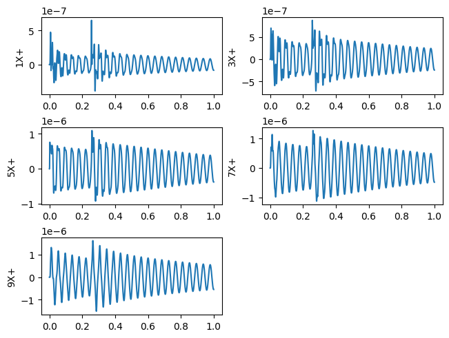
We can then visualize the response of the system.
[13]:
responses.plot(one_axis=False,subplots_kwargs={'layout':'constrained'})
[13]:
array([[<Axes: ylabel='1X+'>, <Axes: ylabel='3X+'>],
       [<Axes: ylabel='5X+'>, <Axes: ylabel='7X+'>],
       [<Axes: ylabel='9X+'>, <Axes: >]], dtype=object)
Modal Analysis
With the mass and stiffness matrices, we could solve for the modes of the system by computing the eigensolution. By calling the eigensolution method on the System object, we can automatically compute the modes of the structure. SDynPy will collect the eigenvalues to extract natural frequency of the structure. The shapes will be extracted from the eigenvectors. SDynPy will automatically construct a ShapeArray object for us with the System object’s coordinates mapped to the ShapeArray object, so the bookkeeping is handled automatically. In the eigensolution method, the number of modes to solve for, or the maximum frequency up to which modes should be solved can be specified.
[14]:
modes = system.eigensolution(maximum_frequency = 200)
modes
[14]:
   Index,  Frequency,    Damping,     # DoFs
    (0,),    23.7873,    0.7473%,         10
    (1,),    70.8306,    2.2252%,         10
    (2,),   116.2917,    3.6534%,         10
    (3,),   159.1549,    5.0000%,         10
    (4,),   198.4630,    6.2349%,         10
We can verify that the coordinates of the System object have been transferred successfully.
[15]:
modes[0].coordinate
[15]:
coordinate_array(string_array=
array(['1X+', '2X+', '3X+', '4X+', '5X+', '6X+', '7X+', '8X+', '9X+',
       '10X+'], dtype='<U4'))
[16]:
system.coordinate
[16]:
coordinate_array(string_array=
array(['1X+', '2X+', '3X+', '4X+', '5X+', '6X+', '7X+', '8X+', '9X+',
       '10X+'], dtype='<U4'))
Sometimes, we have a set of modes (for example from a modal test or from a finite element eigensolution) and we would like to construct a modal model that we can apply forces to to compute response. Computing a System object from a ShapeArray object is trivial in SDynPy. We can simply call the ShapeArray.system method, and it will return a System object. This System will be a reduced system.
[17]:
modal_system = modes.system()
We can visualize the structure of this system again by using the spy method.
[18]:
modal_system.spy()
[18]:
array([<Axes: title={'center': 'Output Transformation'}>,
       <Axes: title={'center': 'Internal State Matrices'}>,
       <Axes: title={'center': 'Input Transformation'}>], dtype=object)
Here we see that the internal state of the modal system is now diagonal (this is expected, every degree of freedom in a modal system should be uncoupled, which is why we can treat modes of a system as single-degree-of-freedom oscillators). The input and output transformations are now “full” in that they are the mode shape matrix. Note that there may be some zeros in the mode shape matrix at nodes of the mode shapes, which is why we see degrees of freedom that are not colored black in some of the shapes.
This is now a reduced system, in that there are 10 physical degrees of freedom, but only 5 state degrees of freedom in the system.
[19]:
modal_system
[19]:
System with 10 DoFs (5 internal DoFs)
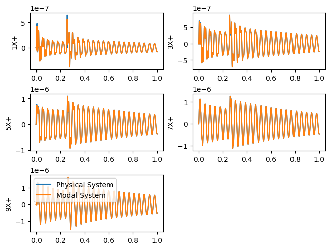
Using a reduced system is essentially identical to using a physical system in SDynPy, however. SDynPy will automatically apply the transformations to forces and responses when doing time integration, and mode shapes will be automatically transformed to physical degrees of freedom when computing the eigensolution.
For example, if we time integrate the modal system with the previous forces, we get almost the identical response, with small differences due to the modal approximation. However, we can see that we are looking at physical response rather than modal response.
[20]:
# Apply forces to the reduced system the same way as the physical system
modal_responses, modal_inputs = modal_system.time_integrate( # Note we are now looking at `modal_system`
    forces, # Same forces as before
    responses = sdpy.coordinate_array(np.arange(1,ndofs+1,2),'X+'), # Only get responses at every other node
    displacement_derivative = 0, # Get displacements out
)

axes = responses.plot(one_axis=False,subplots_kwargs={'layout':'constrained'})
for ax,modal_response in zip(axes.flatten(), modal_responses):
    modal_response.plot(ax)
ax.legend(['Physical System','Modal System'])
[20]:
<matplotlib.legend.Legend at 0x22a65a45160>
Extracting State Space Equations
SDynPy represents its systems using mass, stiffness, and damping matrices. However other tools may represent data differently. One popular format is to represent the system in so-called State Space form, with matrices \(\mathbf{A}\), \(\mathbf{B}\), \(\mathbf{C}\), and \(\mathbf{D}\). SDynPy can produce these matrices from a System object using its to_state_space method. The output degrees of freedom can be selected by passing arguments to the method.
[21]:
A,B,C,D = system.to_state_space(
    output_displacement = True,
    output_velocity = False,
    output_acceleration = False,
    output_force = True,
    response_coordinates = sdpy.coordinate_array(np.arange(1,ndofs+1,2),'X+'), # Only get responses at every other node
    input_coordinates = force_locations[...,0]
    )

print('A Shape {:}\nB Shape {:}\nC Shape {:}\nD Shape {:}'.format(
    A.shape, B.shape, C.shape, D.shape
))
A Shape (20, 20)
B Shape (20, 2)
C Shape (7, 20)
D Shape (7, 2)
We see the proper shapes of the arrays. The state matrix A should have number of rows and columns equal to 2 times the number of degrees of freedom, due to representing displacement and velocity as separate states. The input matrix B should have number of rows equal to 2 times the number of states and number of columns equal to the number of inputs, which in this case is 2. The output matrix C and feedforward matrix D have number of rows equal to the number of outputs, which in this case, we specified as the displacements (of which there are 5) and the forces (of which there are 2). The number of columns of C should match the number of states, and the number of columns of D should match the number of inputs.
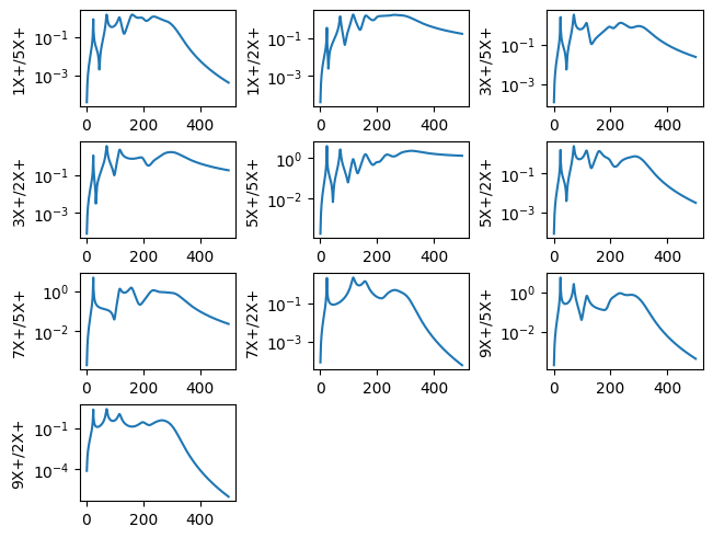
Computing Frequency Response
With a System object, we can compute the frequency response of the structure. We must pass the frequency lines at which the frequency response should be computed. We must also pass the response and reference degrees of freedom to compute the response between, as well as the displacement derivative to specify the type of frequency response function (displacement/force, velocity/force, or acceleration/force).
[22]:
frfs = system.frequency_response(
    np.arange(500)+1,
    responses = sdpy.coordinate_array(np.arange(1,ndofs+1,2),'X+'),
    references = force_locations[...,0],
    displacement_derivative = 2 # Acceleration / force
)

frfs.plot(one_axis=False,subplots_kwargs = {'layout':'constrained'})
[22]:
array([[<Axes: ylabel='1X+/5X+'>, <Axes: ylabel='1X+/2X+'>,
        <Axes: ylabel='3X+/5X+'>],
       [<Axes: ylabel='3X+/2X+'>, <Axes: ylabel='5X+/5X+'>,
        <Axes: ylabel='5X+/2X+'>],
       [<Axes: ylabel='7X+/5X+'>, <Axes: ylabel='7X+/2X+'>,
        <Axes: ylabel='9X+/5X+'>],
       [<Axes: ylabel='9X+/2X+'>, <Axes: >, <Axes: >]], dtype=object)
Beam Finite Elements
SDynPy has a simple set of beam finite elements built in, which allows users to quickly set up small models with realistic physics to play around with. This capability is accessed through the beam class method. This will return both a System object as well as its corresponding Geometry. Material properties can be specified directly, or an optional material argument allows passing the strings 'steel or 'aluminum', which will automatically set the material properties to a standard model of these materials. The material properties set by passing these strings will assume an SI unit system with the beam dimensions specified in meters. Elastic modulus will then be in \(N/m^2\) and density in \(kg/m^3\).
[23]:
beam_system, beam_geometry = sdpy.System.beam(
    length = 1.0,
    width = 0.02,
    height = 0.03,
    num_nodes = 100,
    material = 'steel')
System objects produced by this function will have six degrees of freedom per node (three rotations and three translations).
[24]:
beam_system
[24]:
System with 600 DoFs (600 internal DoFs)
By providing a Geometry along with the System object, SDynPy makes it relatively easy to verify output from analyses.
[25]:
beam_modes = beam_system.eigensolution()
beam_geometry.plot_shape(beam_modes)
[25]:
<sdynpy.core.sdynpy_geometry.ShapePlotter at 0x22a6cea6ba0>

Assigning Damping
Many types of analyses will produce mass and stiffness matrices, but not damping matrices. Damping is difficult to model from first principles, therefore it is often easier to assign it to the model after some measurement or approximation. For example, our beam_system currently has no damping assigned to it.
[26]:
# Check if there are any non-zero terms in the damping matrix
np.any(beam_system.damping != 0)
[26]:
np.False_
While the damping matrix can always be updated to whatever quantities are needed, SDynPy also has two approaches to assign standard damping models to a System object.
Proportional damping is the case where the damping matrix is some linear combination of the stiffness and mass matrices. This is a convenient damping approach to use because the damping matrix will also be exactly diagonalizable from the real modes of the structure computed from an eigensolution, even if it is not a terribly accurate model. We can assign damping in this way using the set_proportional_damping method.
[27]:
beam_system.set_proportional_damping(10,0.1)
We can then see that the damping matrix is made from the mass and stiffness matrices multiplied by the specified coefficients.
[28]:
# Check if the damping is close (to within floating point accuracy) to the
# mass and stiffness matrices times the coefficients.
np.allclose(beam_system.damping, 10*beam_system.mass + 0.1*beam_system.stiffness)
[28]:
True
A second approach to assigning damping is to assign modal damping using the assign_modal_damping method.
[29]:
beam_system.assign_modal_damping(0.02)
This will assign the damping such that when the eigensolution of the system is computed, the modal damping will be the specified values.
[30]:
beam_system.eigensolution(num_modes = 20)
[30]:
   Index,  Frequency,    Damping,     # DoFs
    (0,),     0.0000,    0.0000%,        600
    (1,),     0.0000,    0.0000%,        600
    (2,),     0.0000,    0.0000%,        600
    (3,),     0.0000,    0.0000%,        600
    (4,),     0.0000,    0.0000%,        600
    (5,),     0.0000,    0.0000%,        600
    (6,),   103.7694,    2.0000%,        600
    (7,),   155.6541,    2.0000%,        600
    (8,),   286.0444,    2.0000%,        600
    (9,),   429.0667,    2.0000%,        600
   (10,),   560.7615,    2.0000%,        600
   (11,),   841.1423,    2.0000%,        600
   (12,),   926.9674,    2.0000%,        600
   (13,),  1384.7299,    2.0000%,        600
   (14,),  1390.4512,    2.0000%,        600
   (15,),  1934.0455,    2.0000%,        600
   (16,),  2060.7379,    2.0000%,        600
   (17,),  2077.0949,    2.0000%,        600
   (18,),  2523.8782,    2.0000%,        600
   (19,),  2574.9151,    2.0000%,        600
Note that the rigid body modes with zero frequency cannot have a mode with 2% damping, so they remain zero. All other modes, however, have the specified damping value.
Note that when assigning modal damping, the damping matrix will tend to be “full” rather than “sparse”. The modal damping computation simply finds a form of the damping matrix that satisifies the modal equations. It does not try to respect degree of freedom connectivity. We can visualize this using spy.
[31]:
beam_system.spy()
[31]:
array([<Axes: title={'center': 'Output Transformation'}>,
       <Axes: title={'center': 'Internal State Matrices'}>,
       <Axes: title={'center': 'Input Transformation'}>], dtype=object)
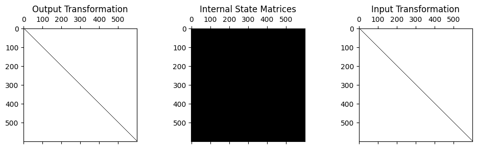
The “full” internal state matrices implies that the degrees of freedom on one end of the beam are directly connected to those on the other side of the beam, which could be viewed as unrealistic as the two ends of the beam are not connected to one another except through the other degrees of freedom in the beam.
Model Reduction
SDynPy provides some standard approaches to model reduction. It implements three reduction strategies, Guyan reduction, Dynamic reduction, and Craig-Bampton reduction, in addition to the modal reduction described previously. See the Example Problem Model Reduction for examples on how to use these methods in a more complicated example.
For Guyan reduction, we simply specify which degrees of freedom to keep in the reduced model and pass them to the reduce_guyan method. Here we keep only the translations at every fifth node, resulting in a factor of 10 reduction in size of the reduced model.
[32]:
dofs_to_keep = sdpy.coordinate_array(
    beam_geometry.node.id[::5],
    ['X+','Y+','Z+'],
    force_broadcast=True
)

beam_system_guyan = beam_system.reduce_guyan(dofs_to_keep)

beam_system_guyan_modes = beam_system_guyan.eigensolution(num_modes=20)
We can compare the modes we get from the reduced model to the full model to judge its accuracy.
[33]:
beam_system_modes = beam_system.eigensolution(num_modes=20)

# Adjust modes because Guyan reduction loses a rigid body mode (rotation about beam)
# due to not keeping rotational dofs.
print(sdpy.shape.shape_comparison_table(beam_system_modes[6:], beam_system_guyan_modes[5:-1]))
  Mode  Freq 1 (Hz)  Freq 2 (Hz)  Freq Error  Damp 1  Damp 2  Damp Error  MAC
     1       103.77       103.77       -0.0%   2.00%   2.00%        0.0%  100
     2       155.65       155.66       -0.0%   2.00%   2.00%        0.0%  100
     3       286.04       286.07       -0.0%   2.00%   2.00%        0.0%  100
     4       429.07       429.11       -0.0%   2.00%   2.00%        0.0%  100
     5       560.76       560.96       -0.0%   2.00%   2.00%        0.0%  100
     6       841.14       841.44       -0.0%   2.00%   2.00%        0.0%  100
     7       926.97       927.84       -0.1%   2.00%   2.00%        0.1%  100
     8      1384.73      1387.58       -0.2%   2.00%   2.00%        0.2%  100
     9      1390.45      1391.77       -0.1%   2.00%   2.00%        0.1%  100
    10      1934.05      1941.62       -0.4%   2.00%   1.99%        0.3%  100
    11      2060.74      2081.37       -1.0%   2.00%   2.00%        0.2%    0
    12      2077.09      2526.75      -17.8%   2.00%   2.00%        0.1%    0
    13      2523.88      2592.32       -2.6%   2.00%   1.99%        0.5%    0
    14      2574.92      2912.42      -11.6%   2.00%   1.99%        0.3%    0
Dynamic reduction is similar to Guyan reduction, except we now also specify a frequency at which we would like the system to match. Guyan reduction (also known as static reduction) is the case of Dynamic reduction where this frequency is zero. We use reduce_dynamic for Dynamic reduction.
[34]:
beam_system_dynamic = beam_system.reduce_dynamic(dofs_to_keep, 1384.73) # Use the 8th mode's frequency

beam_system_dynamic_modes = beam_system_dynamic.eigensolution(num_modes=20)

print(sdpy.shape.shape_comparison_table(beam_system_modes[6:], beam_system_dynamic_modes[5:-1]))
  Mode  Freq 1 (Hz)  Freq 2 (Hz)  Freq Error  Damp 1  Damp 2  Damp Error  MAC
     1       103.77       148.12      -29.9%   2.00%   1.22%       64.0%   94
     2       155.65       168.52       -7.6%   2.00%   1.82%        9.6%  100
     3       286.04       301.77       -5.2%   2.00%   1.88%        6.6%   99
     4       429.07       432.83       -0.9%   2.00%   1.98%        0.9%  100
     5       560.76       566.45       -1.0%   2.00%   1.98%        1.0%  100
     6       841.14       842.04       -0.1%   2.00%   2.00%        0.1%  100
     7       926.97       928.40       -0.2%   2.00%   2.00%        0.1%  100
     8      1384.73      1384.73        0.0%   2.00%   2.00%       -0.0%  100
     9      1390.45      1390.45       -0.0%   2.00%   2.00%        0.0%  100
    10      1934.05      1935.93       -0.1%   2.00%   2.00%        0.1%  100
    11      2060.74      2078.45       -0.9%   2.00%   2.00%        0.1%    0
    12      2077.09      2525.28      -17.7%   2.00%   2.00%        0.1%    0
    13      2523.88      2584.06       -2.3%   2.00%   2.00%        0.3%    0
    14      2574.92      2907.97      -11.5%   2.00%   2.00%        0.2%    0
We see that we have have exactly matched elastic mode 8 by assigning the frequency used in the reduction to that mode’s natural frequency, at the expense of accuracy of other modes.
Perhaps the most popular reduction technique is the Craig-Bampton reduction. In this case, we use a set of fixed interface modes and a set of static deflection modes at the interface. To use this reduction in SDynPy, we must specify the interface degrees of freedom as well as the number of fixed interface modes to keep. We pass this information to the reduce_craig_bampton method.
[35]:
connection_dofs = sdpy.coordinate_array(
    beam_geometry.node.id[[0,-1]],
    ['X+','Y+','Z+','RX+','RY+','RZ+'],
    force_broadcast = True)

beam_system_cb = beam_system.reduce_craig_bampton(connection_dofs,30)
For more complex reductions, it can be illustrative to visualize the shapes used in the transformation. Particularly for the Craig-Bampton reduction, these shapes should look physical; they should be fixed interface modes (modes where the connection degrees of freedom are set to zero, but the rest of the structure can move) and static deflection modes at the interface (modes where a single interface degree of freedom is moved one unit and the rest of the interface degrees of freedom are fixed). We can transform the transformation matrix into a ShapeArray object using the transformation_shapes method.
[36]:
cb_shapes = beam_system_cb.transformation_shapes()

beam_geometry.plot_shape(cb_shapes)
[36]:
<sdynpy.core.sdynpy_geometry.ShapePlotter at 0x22a6d0ef020>
Here we see a one of the fixed-interface modes.

And here is a static deflection mode of the interface.

[37]:
beam_system_cb_modes = beam_system_cb.eigensolution(num_modes=20)

print(sdpy.shape.shape_comparison_table(beam_system_modes[6:], beam_system_cb_modes[6:]))
  Mode  Freq 1 (Hz)  Freq 2 (Hz)  Freq Error  Damp 1  Damp 2  Damp Error  MAC
     1       103.77       103.77       -0.0%   2.00%   2.00%        0.0%  100
     2       155.65       155.66       -0.0%   2.00%   2.00%        0.0%  100
     3       286.04       286.05       -0.0%   2.00%   2.00%        0.0%  100
     4       429.07       429.08       -0.0%   2.00%   2.00%        0.0%  100
     5       560.76       560.79       -0.0%   2.00%   2.00%        0.0%  100
     6       841.14       841.31       -0.0%   2.00%   2.00%        0.0%  100
     7       926.97       927.11       -0.0%   2.00%   2.00%        0.0%  100
     8      1384.73      1385.03       -0.0%   2.00%   2.00%        0.0%  100
     9      1390.45      1390.87       -0.0%   2.00%   2.00%        0.0%  100
    10      1934.05      1934.97       -0.0%   2.00%   2.00%        0.0%  100
    11      2060.74      2062.85       -0.1%   2.00%   2.00%        0.1%  100
    12      2077.09      2078.69       -0.1%   2.00%   2.00%        0.1%  100
    13      2523.88      2535.12       -0.4%   2.00%   1.99%        0.3%  100
    14      2574.92      2576.32       -0.1%   2.00%   2.00%        0.0%  100
We see that the Craig-Bampton reduction performs better than the Guyan and Dynamic reduction even though it has fewer remaining degrees of freedom.
[38]:
beam_system_guyan
[38]:
System with 600 DoFs (60 internal DoFs)
[39]:
beam_system_cb
[39]:
System with 600 DoFs (42 internal DoFs)
One key takeaway is that when working with reduced systems, the user does not need to expend effort managing the bookkeeping associated with the reduction transformation. The transformation is handled seamlessly whenever data is requested. When computing modes, the resulting ShapeArray was already presented in physical degrees of freedom rather than in some underlying state degrees of freedom.
Substructuring and Applying Constraints
When working with System objects, sometimes we would like to assemble larger systems from smaller subsystems. SDynPy offers tools to aid in performing these operations. Let’s create three beam objects and investigate how we can perform these substructuring operations.
[40]:
left_beam, left_beam_geometry = sdpy.System.beam(0.1,0.01,0.01, num_nodes = 10, material='steel')
right_beam, right_beam_geometry = sdpy.System.beam(0.1,0.01,0.01, num_nodes = 10, material='steel')
center_beam, center_beam_geometry = sdpy.System.beam(0.5,0.01,0.01, num_nodes = 50, material='steel')
Since we will be combining the beams together, let’s go ahead and overlay the beam geometries to combine them into one object. We will use the Geometry.overlay_geometries function, and ensure that we return_node_id_offset so we can apply the same node offset to our System objects.
[41]:
combined_geometry, node_offset = sdpy.Geometry.overlay_geometries(
    geometries = [left_beam_geometry,center_beam_geometry,right_beam_geometry],
    color_override = [1,5,11], # Blue, green, red
    return_node_id_offset = True
    )

combined_geometry.plot()
[41]:
(<sdynpy.core.sdynpy_geometry.GeometryPlotter at 0x22a659ccb00>,
 PolyData (0x22a6de0c760)
   N Cells:    3
   N Points:   70
   N Strips:   0
   X Bounds:   0.000e+00, 5.000e-01
   Y Bounds:   0.000e+00, 0.000e+00
   Z Bounds:   0.000e+00, 0.000e+00
   N Arrays:   1,
 PolyData (0x22a6de0cbe0)
   N Cells:    70
   N Points:   70
   N Strips:   0
   X Bounds:   0.000e+00, 5.000e-01
   Y Bounds:   0.000e+00, 0.000e+00
   Z Bounds:   0.000e+00, 0.000e+00
   N Arrays:   2,
 None)

Currently, all the beams are on top of one another, so we should shift them around. We can easily do this by modifying their coordinate systems. We will compute a rotation matrix using the R function to provide a 90 degree rotation about Y. We will them apply that to the coordinate systems of the left and right beams.
[42]:
# Rotate 90 degrees about Y
rotation_matrix = sdpy.rotation.R(1,90,'degrees')

# We are looking to get the first three rows of the first and last
# coordinate systems
combined_geometry.coordinate_system.matrix[[0,-1],:3,:] = rotation_matrix
We will then translate one of the coordinate systems so it lies at the other end of the beam.
[43]:
translation_vector = np.array([0.5,0,0])[:,np.newaxis]

# We are looking to get the last row of the first coordinate system
combined_geometry.coordinate_system.matrix[0, 3:,:] = translation_vector[:,0]

combined_geometry.plot()
[43]:
(<sdynpy.core.sdynpy_geometry.GeometryPlotter at 0x22a6de07920>,
 PolyData (0x22a6de0de40)
   N Cells:    3
   N Points:   70
   N Strips:   0
   X Bounds:   0.000e+00, 5.000e-01
   Y Bounds:   0.000e+00, 0.000e+00
   Z Bounds:   0.000e+00, 1.000e-01
   N Arrays:   1,
 PolyData (0x22a6de0e6e0)
   N Cells:    70
   N Points:   70
   N Strips:   0
   X Bounds:   0.000e+00, 5.000e-01
   Y Bounds:   0.000e+00, 0.000e+00
   Z Bounds:   0.000e+00, 1.000e-01
   N Arrays:   2,
 None)

With the geometry now set up, we will focus on our System objects. The first thing we will do is combine them into a single System object. We can do this using the System.concatenate method. This method takes an optional offset parameter, which is exactly the parameter we received from the Geometry.overlay_geometries method.
[44]:
combined_system = sdpy.System.concatenate(
    systems = [left_beam, center_beam, right_beam],
    coordinate_node_offset = node_offset
)
We see that if we look at the Geometry node identification numbers and the System coordinates, they contain the same node numbers.
[45]:
combined_geometry.node
[45]:
   Index,     ID,        X,        Y,        Z, DefCS, DisCS
    (0,),    101,    0.000,    0.000,    0.000,    11,    11
    (1,),    102,    0.011,    0.000,    0.000,    11,    11
    (2,),    103,    0.022,    0.000,    0.000,    11,    11
    (3,),    104,    0.033,    0.000,    0.000,    11,    11
    (4,),    105,    0.044,    0.000,    0.000,    11,    11
    (5,),    106,    0.056,    0.000,    0.000,    11,    11
    (6,),    107,    0.067,    0.000,    0.000,    11,    11
    (7,),    108,    0.078,    0.000,    0.000,    11,    11
    (8,),    109,    0.089,    0.000,    0.000,    11,    11
    (9,),    110,    0.100,    0.000,    0.000,    11,    11
   (10,),    201,    0.000,    0.000,    0.000,    21,    21
   (11,),    202,    0.010,    0.000,    0.000,    21,    21
   (12,),    203,    0.020,    0.000,    0.000,    21,    21
   (13,),    204,    0.031,    0.000,    0.000,    21,    21
   (14,),    205,    0.041,    0.000,    0.000,    21,    21
   (15,),    206,    0.051,    0.000,    0.000,    21,    21
   (16,),    207,    0.061,    0.000,    0.000,    21,    21
   (17,),    208,    0.071,    0.000,    0.000,    21,    21
   (18,),    209,    0.082,    0.000,    0.000,    21,    21
   (19,),    210,    0.092,    0.000,    0.000,    21,    21
   (20,),    211,    0.102,    0.000,    0.000,    21,    21
   (21,),    212,    0.112,    0.000,    0.000,    21,    21
   (22,),    213,    0.122,    0.000,    0.000,    21,    21
   (23,),    214,    0.133,    0.000,    0.000,    21,    21
   (24,),    215,    0.143,    0.000,    0.000,    21,    21
   (25,),    216,    0.153,    0.000,    0.000,    21,    21
   (26,),    217,    0.163,    0.000,    0.000,    21,    21
   (27,),    218,    0.173,    0.000,    0.000,    21,    21
   (28,),    219,    0.184,    0.000,    0.000,    21,    21
   (29,),    220,    0.194,    0.000,    0.000,    21,    21
   (30,),    221,    0.204,    0.000,    0.000,    21,    21
   (31,),    222,    0.214,    0.000,    0.000,    21,    21
   (32,),    223,    0.224,    0.000,    0.000,    21,    21
   (33,),    224,    0.235,    0.000,    0.000,    21,    21
   (34,),    225,    0.245,    0.000,    0.000,    21,    21
   (35,),    226,    0.255,    0.000,    0.000,    21,    21
   (36,),    227,    0.265,    0.000,    0.000,    21,    21
   (37,),    228,    0.276,    0.000,    0.000,    21,    21
   (38,),    229,    0.286,    0.000,    0.000,    21,    21
   (39,),    230,    0.296,    0.000,    0.000,    21,    21
   (40,),    231,    0.306,    0.000,    0.000,    21,    21
   (41,),    232,    0.316,    0.000,    0.000,    21,    21
   (42,),    233,    0.327,    0.000,    0.000,    21,    21
   (43,),    234,    0.337,    0.000,    0.000,    21,    21
   (44,),    235,    0.347,    0.000,    0.000,    21,    21
   (45,),    236,    0.357,    0.000,    0.000,    21,    21
   (46,),    237,    0.367,    0.000,    0.000,    21,    21
   (47,),    238,    0.378,    0.000,    0.000,    21,    21
   (48,),    239,    0.388,    0.000,    0.000,    21,    21
   (49,),    240,    0.398,    0.000,    0.000,    21,    21
   (50,),    241,    0.408,    0.000,    0.000,    21,    21
   (51,),    242,    0.418,    0.000,    0.000,    21,    21
   (52,),    243,    0.429,    0.000,    0.000,    21,    21
   (53,),    244,    0.439,    0.000,    0.000,    21,    21
   (54,),    245,    0.449,    0.000,    0.000,    21,    21
   (55,),    246,    0.459,    0.000,    0.000,    21,    21
   (56,),    247,    0.469,    0.000,    0.000,    21,    21
   (57,),    248,    0.480,    0.000,    0.000,    21,    21
   (58,),    249,    0.490,    0.000,    0.000,    21,    21
   (59,),    250,    0.500,    0.000,    0.000,    21,    21
   (60,),    301,    0.000,    0.000,    0.000,    31,    31
   (61,),    302,    0.011,    0.000,    0.000,    31,    31
   (62,),    303,    0.022,    0.000,    0.000,    31,    31
   (63,),    304,    0.033,    0.000,    0.000,    31,    31
   (64,),    305,    0.044,    0.000,    0.000,    31,    31
   (65,),    306,    0.056,    0.000,    0.000,    31,    31
   (66,),    307,    0.067,    0.000,    0.000,    31,    31
   (67,),    308,    0.078,    0.000,    0.000,    31,    31
   (68,),    309,    0.089,    0.000,    0.000,    31,    31
   (69,),    310,    0.100,    0.000,    0.000,    31,    31
[46]:
np.unique(combined_system.coordinate.node)
[46]:
array([101, 102, 103, 104, 105, 106, 107, 108, 109, 110, 201, 202, 203,
       204, 205, 206, 207, 208, 209, 210, 211, 212, 213, 214, 215, 216,
       217, 218, 219, 220, 221, 222, 223, 224, 225, 226, 227, 228, 229,
       230, 231, 232, 233, 234, 235, 236, 237, 238, 239, 240, 241, 242,
       243, 244, 245, 246, 247, 248, 249, 250, 301, 302, 303, 304, 305,
       306, 307, 308, 309, 310], dtype=uint64)
Currently, however, this concatenation is simply a bookkeeping exercise. There have been no physical constraints applied to enforce that certain degrees of freedom move together. For example, if we compute the eigensolution of this System, we see that the system is effectively three separate systems.
[47]:
combined_geometry.plot_shape(combined_system.eigensolution())
[47]:
<sdynpy.core.sdynpy_geometry.ShapePlotter at 0x22a6de1d760>

We need to tell the System objects that certain degrees of freedom are equivalent. We can do this easily by specifying pairs of degrees of freedom to glue together. It can be helpful to visualize this using the Geometry.plot_coordinate method.
[48]:
combined_geometry.plot_coordinate(sdpy.coordinate_array(201,['X+','Y+','Z+']), label_dofs=True, arrow_scale=0.02)
combined_geometry.plot_coordinate(sdpy.coordinate_array(301,['X+','Y+','Z+']), label_dofs=True, arrow_scale=0.02)
[48]:
<sdynpy.core.sdynpy_geometry.GeometryPlotter at 0x22a6de2deb0>

We can see from these plots the pairs of degrees of freedom that we must constrain togther. For example, 301X+ is equivalent to 201Z+. Similarly, 301Z+ is equivalent to 201X-. We can construct pairs of these degrees of freedom, keeping in mind we must also constrain rotations as well as the other connection point.
[49]:
dof_pairs_as_strings = [['201Z+','301X+'],
                        ['201Y+','301Y+'],
                        ['201X-','301Z+'],
                        ['250Z+','101X+'],
                        ['250Y+','101Y+'],
                        ['250X-','101Z+'],
                        ['201RZ+','301RX+'],
                        ['201RY+','301RY+'],
                        ['201RX-','301RZ+'],
                        ['250RZ+','101RX+'],
                        ['250RY+','101RY+'],
                        ['250RX-','101RZ+']]

dof_pairs = sdpy.coordinate_array(string_array = dof_pairs_as_strings)

dof_pairs
[49]:
coordinate_array(string_array=
array([['201Z+', '301X+'],
       ['201Y+', '301Y+'],
       ['201X-', '301Z+'],
       ['250Z+', '101X+'],
       ['250Y+', '101Y+'],
       ['250X-', '101Z+'],
       ['201RZ+', '301RX+'],
       ['201RY+', '301RY+'],
       ['201RX-', '301RZ+'],
       ['250RZ+', '101RX+'],
       ['250RY+', '101RY+'],
       ['250RX-', '101RZ+']], dtype='<U6'))
We can then apply the constraints by passing these degree of freedom to the substructure_by_coordinate method.
[50]:
constrained_system = combined_system.substructure_by_coordinate(dof_pairs)
This constrained system has had 12 constraints applied, meaning 12 degrees of freedom have been removed from the System. We can compare the number of degrees of freedom in the original system with the constrained system to verify that the latter has 12 fewer degrees of freedom.
[51]:
constrained_system
[51]:
System with 420 DoFs (408 internal DoFs)
[52]:
combined_system
[52]:
System with 420 DoFs (420 internal DoFs)
Indeed, the combined system has 420 degrees of freedom while the constrained system has 408, which is a difference of 12. We can also verify that the degrees of freedom that have been glued together move together in all of the modes of the system.
[53]:
constrained_modes = constrained_system.eigensolution()

combined_geometry.plot_shape(constrained_modes)
[53]:
<sdynpy.core.sdynpy_geometry.ShapePlotter at 0x22a6de2fd10>

To fix a degree of freedom to allow no motion, we can pair it with None in the same substructure_by_coordinate method. Perhaps we would like the tips of the left and right beams to be fixed in place. One thing to note is that we cannot have None in a CoordinateArray, so we instead must use a list of CoordinateArray objects.
[54]:
fix_dofs = sdpy.coordinate_array([110,310],[1,2,3,4,5,6],force_broadcast=True)

fixed_constraints = [(dof,None) for dof in fix_dofs] + [dof_pair for dof_pair in dof_pairs]

fixed_system = combined_system.substructure_by_coordinate(fixed_constraints)

fixed_modes = fixed_system.eigensolution()

combined_geometry.plot_shape(fixed_modes)
[54]:
<sdynpy.core.sdynpy_geometry.ShapePlotter at 0x22a6de2fda0>

We now see that there is no motion at the tips of the short beams.
More advanced substructuring functionality exists in SDynPy that is outside of the scope of this document. Users are directed to the substructure_by_position method that can automatically detect degree of freedom pairs and perform constraints, even when coordinate systems are not aligned. The substructure_by_shape method can provide “softened” constraints over continuous boundaries, rather than hard constraints at discrete degrees of freedom.
Reading and Writing NumPy Files
SDynPy uses NumPy’s file types to store its data. In the case of a System object, the various mass, stiffness, damping, and transformation matrices are written to separate fields in a NumPy .npz file. Similarly, the coordinate data is also stored to this file.
System objects can be saved using the System.save method. Similarly System objects can be loaded from disk using the System.load class method.
[55]:
# Save the file
fixed_system.save('system.npz')

# Load a saved file
fixed_system_from_npy = sdpy.System.load('system.npz')
Summary
This document described the System object, which is used to represent dynamic systems in SDynPy. The System object can be used to represent physical or reduced systems using the transformation matrix attribute. The transformation is handled seamlessly in operations that request data from the object, with the data automatically being transformed back to physical space, which greatly simplifies bookkeeping operations.
System objects make it easy to simulate response to certain excitations. A TimeHistoryArray can be constructed with the input forces and passed to the time_integrate method to compute responses to that excitation. The frequency response of a System can be computed using the compute_frequency_response method, which will return a TransferFunctionArray containing the requested input and output degrees of freedom.
The modes of a System object can be quickly computed with the eigensolution method, which results in a ShapeArray object. The ShapeArray object can be transformed into a reduced System object by calling its ShapeArray.system method. Reduced systems can also be explicitly constructed from full systems. Methods like reduce_guyan, reduce_dynamic, and reduce_craig_bampton will construct reduced systems with minimal effort from the user.
SDynPy has a limited set of beam finite elements that can be accessed through the System.beam method. These will produce a System object and a corresponding Geometry object which can be used to plot results. Damping can be assigned to these systems by modifying the damping matrix or otherwise calling the assign_modal_damping or set_proportional_damping methods.
SDynPy System objects have a very flexible substructuring and constraint programming interface, allowing for substructuring operations to be performed with minimal bookkeeping effort from the user. Constraints can be applied by directly constraining degrees of freedom to move together or to be fixed using the substructure_by_coordinate method. Constraints can also be applied by position using the substructure_by_position function or by shape using the substructure_by_shape method.
Like most SDynPy objects, the System object can be saved to or loaded from a NumPy file using its save and load methods.