Substructuring using the Transmission Simulator Method
This example will demonstrate the capabilities in SDynPy for performing more advanced substructuring calculations using the Transmission Simulator Method. The transmission simulator method is a useful form of substructuring which allows the interface of the substructures to be mass-loaded, which provides a better set of basis shapes to use in the substructuring calculation.
Contents
Setting up the Problem
We will first use the Cubit software to generate a mesh for the finite element
analysis that will be used in this example problem. We will create a 3-part
model of a box inside of a container. The container is labeled A, the lid is
labeled B, and the internal box is labeled C. The attached input file can
be executed using Cubit’s Python interface to create the model.
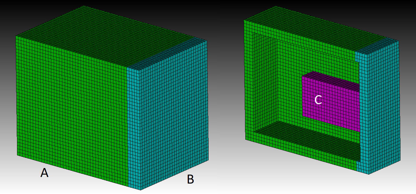
Mesh generated by Cubit shown both in whole and in cross section to reveal the three components.
The model contains 3 element blocks, block 1, block 2, and block 3, which are
the container A, the lid B, and the internal box C, respectively. The attached
input file will generate several exodus files that can be used to investigate
substructuring. Each object will be generated independently, a.exo, b.exo,
and c.exo. Additionally, meshes will be generated for pairs of components,
ab.exo and bc.exo. Finally, a full model abc.exo will be generated which
will provide truth data to compare the substructuring results to.
Input files are then set up for the Sierra/SD code. Each input file will
contain an Eigensolution eigen which will solve for the component modes
used in the substructuring. The input files for each mesh are attached:
When run, these will generate output files containing the natural frequencies and mode shapes of the structures.
To perform the transmission simulator approach, we will add substructure AB
to substructure BC and then subtract off the extra B. In this case, the
structure B serves as the transmission simulator because it mass-loads the
interfaces of A and C to give a better set of basis shapes to use in the
substructuring.
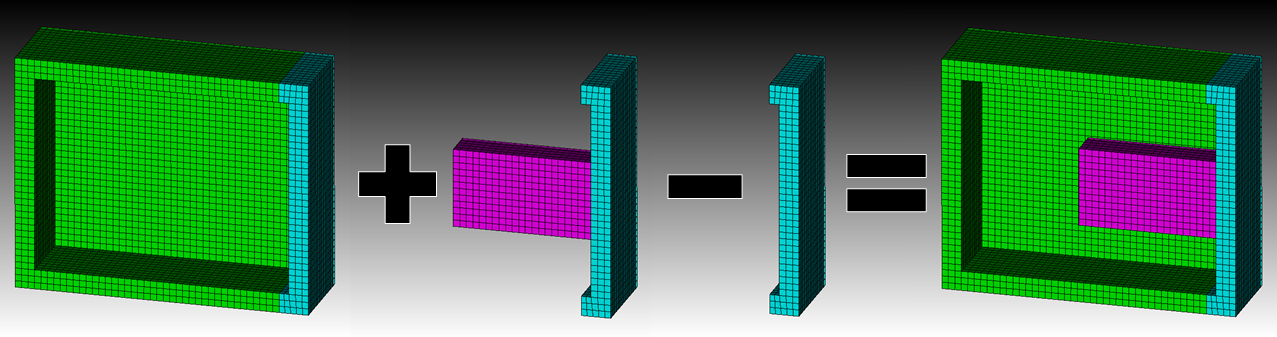
Substructuring operations performed in the transmission simulator method.
The system AB is added to BC and then system B is subtracted to
produce system ABC.
Loading the results into SDynPy
We will now load the models into SDynPy in order to perform the analysis. We will start by importing the required modules and setting up plotting options.
# Import modules
import sdynpy as sdpy # For dynamics
import numpy as np # For numerics
import matplotlib.pyplot as plt # For plotting
from scipy.spatial import QhullError # For creating elements for visualization

# Set up options to use for plotting
plot_options = {'node_size':0,'line_width':1,'show_edges':False,
                'view_up':[0,1,0]}
We will now load in the models and plot their mode shapes to make sure
everything looks right. For each model we will reduce to just the surface
nodes and elements for visualization using the
reduce_to_surfaces
method of the Exodus class.
We will then create Geometry
as well as a Shapes from the
finite element data using the respective
sdpy.geometry.from_exodus and
sdpy.shape.from_exodus methods.
# Specify the models to load into SDynPy
models = ['a','b','c','ab','bc','abc']

# For each model, load in the exodus file and reduce it to surfaces
fexos = {model:sdpy.Exodus(model+'-out.exo').reduce_to_surfaces()
         for model in models}

# For each model create a SDynPy Geometry from the finite element model
geometries = {model:sdpy.Geometry.from_exodus(fexos[model])
              for model in models}

# For each model create a SDynPy ShapeArray from the eigensolution results
shapes = {model:sdpy.shape.from_exodus(fexos[model])
          for model in models}
# For each model, plot the mode shapes on the geometry
for model in models:
    geometries[model].plot_shape(shapes[model],plot_options,
                                 deformed_opacity=0.5,
                                 undeformed_opacity=0)
Mode Shape for System A
Mode Shape for System B
Mode Shape for System C
Mode Shape for System AB
Mode Shape for System BC
Mode Shape for System ABC
Reducing to Test Degrees of Freedom
For this example, we will pretend that the finite element results are actually test data, and for this reason, we will reduce to a more limited set of degrees of freedom in each model that may have been measured in a test. We will first define the geometry of the system so we can select the final kept set of nodes by position.
container_size = [1.0,1.2,1.5]
component_size = [0.4,0.4,0.7]
lid_depth = 0.15
container_thickness = 0.1

lid_position = container_size[-1]/2-lid_depth
component_position = container_size[-1]/2-container_thickness-component_size[-1]/2

grid_size = 3
component_grid_size = 2
grid_inset = 0.1
We will then loop through each face of the model to get sensor positions that we would like to use in the test. We will use NumPy functions linspace and meshgrid. to produce grids of sensors on each surface.
# Loop through each face to get sensor positions
positions = []
indices = []
index = 0
# Outer box
for dimension in range(3):
    other_dimensions = [v for v in range(3) if not v == dimension]
    meshgrid_inputs = [None,None,None]
    grid_0 = container_size[dimension]/2
    grid_1 = np.linspace(-container_size[other_dimensions[0]]/2+grid_inset,
                          container_size[other_dimensions[0]]/2-grid_inset,
                          grid_size)
    grid_2 = np.linspace(-container_size[other_dimensions[1]]/2+grid_inset,
                          container_size[other_dimensions[1]]/2-grid_inset,
                          grid_size)
    meshgrid_inputs[dimension] = grid_0
    meshgrid_inputs[other_dimensions[0]] = grid_1
    meshgrid_inputs[other_dimensions[1]] = grid_2
    this_positions = np.moveaxis(np.array(np.meshgrid(*meshgrid_inputs,indexing='ij')).squeeze(),0,-1).reshape(-1,3)
    positions.append(this_positions)
    indices.append(np.ones(this_positions.shape[0])*index)
    index += 1
    # Now do the negative side
    this_positions_opposite = this_positions.copy()
    this_positions_opposite[...,dimension] *= -1
    positions.append(this_positions_opposite)
    indices.append(np.ones(this_positions.shape[0])*index)
    index += 1
# Component box
for dimension in range(2):
    other_dimensions = [v for v in range(3) if not v == dimension]
    meshgrid_inputs = [None,None,None]
    grid_0 = component_size[dimension]/2
    grid_1 = np.linspace(-component_size[other_dimensions[0]]/2+grid_inset,
                          component_size[other_dimensions[0]]/2-grid_inset,
                          component_grid_size)
    grid_2 = np.linspace(-component_size[other_dimensions[1]]/2+grid_inset+component_position,
                          component_size[other_dimensions[1]]/2-grid_inset+component_position,
                          component_grid_size)
    meshgrid_inputs[dimension] = grid_0
    meshgrid_inputs[other_dimensions[0]] = grid_1
    meshgrid_inputs[other_dimensions[1]] = grid_2
    this_positions = np.moveaxis(np.array(np.meshgrid(*meshgrid_inputs,indexing='ij')).squeeze(),0,-1).reshape(-1,3)
    positions.append(this_positions)
    indices.append(np.ones(this_positions.shape[0])*index)
    index += 1
    # Now do the negative side
    this_positions_opposite = this_positions.copy()
    this_positions_opposite[...,dimension] *= -1
    positions.append(this_positions_opposite)
    indices.append(np.ones(this_positions.shape[0])*index)
    index += 1

positions = np.concatenate(positions,axis=0)
indices = np.concatenate(indices,axis=0)
We will now reduce each of the geometries down to its test sensors using
the reduce method,
using the by_position
method of the NodeArray
object to select which nodes to keep. Note that this will simply select the
closest node to the position specified, which isn’t exactly what we want. For
example, if a position is specified that corresponds to a node on system A,
but the system we are generating test data for is system BC (which doesn’t
contain system A) it will instead select a node the closest node on BC
to that point, rather than simply not selecting a node at all. We will discard
these points and connect the test nodes with elements and tracelines to ease
visualization.
We will specify a distance threshold to compare the point where we wanted to
select a node and where the closest node was selected, and use that to discard
improperly selected nodes. We will also specify a maximum condition number for
triangles created as elements for visualization. We will also set up a
dictionary of id_map objects
to map the nodes between the test geometry and the finite element model.
distance_threshold = 0.05
max_condition = 10
node_id_maps = {}
We will then loop through all of our test geometries and finish their creation.
# Now create the test geometries
for model in test_geometries:
    print('Creating test geometry for {:}'.format(model))
Within this loop, we will set up a node map from the finite element model nodes to the test nodes, which will be labeled 1 through $n_nodes$ for each system, where $n_nodes$ is the number of nodes for each test geometry.
geometry = test_geometries[model]
from_ids = geometry.node.id
to_ids = np.arange(geometry.node.size)+1
node_id_maps[model] = sdpy.id_map(from_ids, to_ids)
At this point, we will now discard the nodes that aren’t close enough to their desired positions, and then use the node map to rename the nodes in the model.
# Throw away nodes that aren't in the model
distance = np.linalg.norm(geometry.node.coordinate-positions,axis=-1)
keep_indices = distance < distance_threshold
new_geometry = geometry.reduce(geometry.node.id[keep_indices])
new_geometry.node.id = node_id_maps[model](new_geometry.node.id)
original_indices = indices[keep_indices]
We will then add elements using the
triangulate method
of the NodeArray object. If
the nodes cannot be triangulated, they are instead connected with a traceline.
# Create elements
elements = []
for value in np.unique(original_indices):
    face_indices = original_indices == value
    face_nodes = new_geometry.node[face_indices]
    try:
        face_elements = face_nodes.triangulate(new_geometry.coordinate_system,
                                               condition_threshold=max_condition)
        elements.append(np.atleast_1d(face_elements))
    except QhullError:
        new_geometry.add_traceline(face_nodes.id)
new_geometry.element = np.concatenate(elements)
new_geometry.element.id = np.arange(new_geometry.element.size)+1
test_geometries[model] = new_geometry
We can then similarly map the shapes to the new test geometries. We will use
the
transform_coordinate_system
method of the ShapeArray object
to simultaneously reduce the shape down to the test geometry and apply the
node map. We will also assign a 1% damping to each of the test shapes. We will
plot the reduced shapes as well as a MAC matrix to ensure the shapes are still
distinguishable in their reduced form.
# Now create the test shapes
test_shapes = {}
for model in shapes:
    print('Creating test shapes for {:}'.format(model))
    shape = shapes[model]
    original_geometry = geometries[model]
    new_geometry = test_geometries[model]
    id_map = node_id_maps[model]
    test_shape = shape.transform_coordinate_system(original_geometry,new_geometry,id_map)
    test_shape.damping = 0.01
    test_shapes[model] = test_shape
    test_geometries[model].plot_shape(test_shapes[model],plot_options,undeformed_opacity=0,deformed_opacity=0.5)
    sdpy.correlation.matrix_plot(sdpy.shape.mac(test_shapes[model]))
Test Mode Shape for System A
Test Mode Shape for System B
Test Mode Shape for System C
Test Mode Shape for System AB
Test Mode Shape for System BC
Test Mode Shape for System ABC
Substructuring using the Transmission Simulator Method
Now that we have our models set up, we can proceed with the substructuring.
We will define our bandwidth as 2000 Hz, and select to use 15 transmission
simulator modes to perform the substructuring. We can then reduce down to
just the shapes satisfying these critera, and create modal
System from them. This will
result in diagonal mass, stiffness, and damping matrices, with the mode shape
matrix as the transformation to physical coordinates.
Recall, we will be attempting to compute system ABC from components AB,
BC, and B.
bandwidth = 2000
transmission_simulator_modes = 15
system_ab = test_shapes['ab'][test_shapes['ab'].frequency < bandwidth].system()
system_bc = test_shapes['bc'][test_shapes['bc'].frequency < bandwidth].system()
system_b = test_shapes['b'][:transmission_simulator_modes].system()
The first step is to combine the components AB, BC, and B into one
System object. Note that no
constraints have been applied, so the system matrices will be block diagonal.
We will also combine the geometries so we can eventually plot mode shapes of
the combined system. We will combine the geometries first, as it will give us
a node offset that we can use to avoid conflicting nodes in the various
substructures using the
overlay_geometries
static method of the Geometry
object. We pass it a list of geometries to combine, a set of colors to make
each geometry, as well as tell it to return the node offset used to avoid
conflicts. We will then combine the systems using the
concatenate static
method of the System object
to combine the systems, passing the node offset as an argument to keep the
concatenated systems consistent with the combined geometries. Note that because
we will be subtracting component B from the assembly, we will specify a
negative system_b during the concatenation. We can use the
System.spy method to visualize
the structure of the created system and ensure that it is block-diagonal.
geoms = (test_geometries['ab'],test_geometries['bc'],test_geometries['b'])
combined_geometry,node_offset = sdpy.Geometry.overlay_geometries(
    geoms,
    color_override=[1,7,11],
    return_node_id_offset=True)
systems = (system_ab,system_bc,-system_b) # Note that system_b is negative
combined_system = sdpy.System.concatenate(
    systems,node_offset)
combined_system.spy()
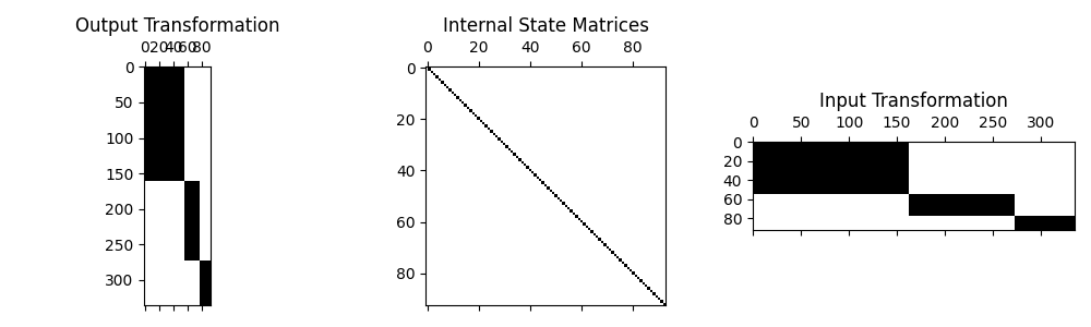
Structure of the concatenated system, showing block-diagonal structure.
If we were to plot this concatenated system’s modes, it would be like we just
overlaid all three systems on top of one another. This is because no constraints
have yet been applied, so, e.g., component AB has no effect on component
BC.
combined_geometry.plot_shape(combined_system.eigensolution(),plot_options)
Note however, that this will not work in its current state, due to the negative
mass on component B. If we instead flip B to positive and re-run the
previous code block, we can then plot the shapes. If you do this, don’t forget
to flip the sign back to negative, otherwise the substructuring won’t work!
Mode Shape for System B in the concatenated system
Mode Shape for System AB in the concatenated system
Mode Shape for System BC in the concatenated system
Finally, we can apply constraints to the model. We will first find the nodes
that are used in the constraint. These will be the nodes in B that are also
in AB. We will create another set of
id_map objects to map the
degrees of freedom from the original test geometries to the combined test
geometry, which has the node offset applied.
connection_nodes = np.intersect1d(test_geometries['ab'].node.id,test_geometries['b'].node.id)
connection_map_ab = sdpy.id_map(connection_nodes,connection_nodes + node_offset)
connection_map_bc = sdpy.id_map(connection_nodes,connection_nodes + node_offset*2)
connection_map_b = sdpy.id_map(connection_nodes,connection_nodes + node_offset*3)
Because the transmission simulator method uses softened, least-squares constraints, we must also construct the basis set of shapes used in the constraint. These will be the mode shapes of the transmission simulator mapped to the nodes in the combined system for each substructure. To help verify that they are assembled correctly, these shapes can be plotted on the combined geometry. If degrees of freedom have been correctly selected for each constraint, the boundary nodes of the substructures should be seen to move identically in each shape.
connection_shapes_ab = test_shapes['b'][:transmission_simulator_modes].copy()
connection_shapes_ab.coordinate.node = connection_map_ab(connection_shapes_ab.coordinate.node)
connection_shapes_bc = test_shapes['b'][:transmission_simulator_modes].copy()
connection_shapes_bc.coordinate.node = connection_map_bc(connection_shapes_bc.coordinate.node)
connection_shapes_b = test_shapes['b'][:transmission_simulator_modes].copy()
connection_shapes_b.coordinate.node = connection_map_b(connection_shapes_b.coordinate.node)
# Combine all the shape degrees of freedom into one shape
connection_shapes = sdpy.shape.concatenate_dofs([connection_shapes_ab,connection_shapes_bc,connection_shapes_b])

# Now to make sure this is correct, if we plot these shapes on the combined
# geometry, it should move all of the connection degrees of freedom in the
# shapes of the transmission simulator
combined_geometry.plot_shape(connection_shapes,plot_options,deformed_opacity=0.5,
                             undeformed_opacity=0)
Once we have these shapes, we can select the coordinates in each system
in each shape and then create the constraint matrix using the
substructure_by_shape
method of the System object.
To this method get passed the shapes to use as the basis for the constraints
as well as the degrees of freedom to use in each system for the computation of
the least-squares constraint. This method could directly return a constrained
system, but instead we set the argument return_constrained_system=False,
which instead makes the method return the constraint matrix instead. We
do this because we will be applying another set of shape constraints for the
other substructure, and wish to apply the constraints all at once.
connection_dofs_ab = combined_system.coordinate[np.in1d(combined_system.coordinate.node,
                                                        connection_map_ab.to_ids)]
connection_dofs_bc = combined_system.coordinate[np.in1d(combined_system.coordinate.node,
                                                        connection_map_bc.to_ids)]
connection_dofs_b = combined_system.coordinate[np.in1d(combined_system.coordinate.node,
                                                        connection_map_b.to_ids)]

constraint_matrix_ab_b = combined_system.substructure_by_shape(connection_shapes,
                                                          connection_dofs_ab,
                                                          connection_dofs_b,
                                                          return_constrained_system=False)
constraint_matrix_bc_b = combined_system.substructure_by_shape(connection_shapes,
                                                          connection_dofs_bc,
                                                          connection_dofs_b,
                                                          return_constrained_system=False)
Note that all of the bookkeeping is handled automatically by the
substructure_by_shape
method, we simply had to specify which degrees of freedom were to be used in the
substructuring, and ensure that those degrees of freedom existed in the shapes
used for the modal constraints.
We can then concatenate the two constraint matrices into a single constraint
matrix and apply it to the system using the
constrain
method of the System object.
constraint_matrix = np.concatenate((constraint_matrix_ab_b,constraint_matrix_bc_b),axis=0)

constrained_system = combined_system.constrain(constraint_matrix)
We can then solve for the modes of the constrained system, and compare them against the truth shapes from the full finite element model.
constrained_shapes = constrained_system.eigensolution()

combined_geometry.plot_shape(constrained_shapes,plot_options,deformed_opacity=0.5,
                             undeformed_opacity=0.0)

test_geometries['abc'].plot_shape(test_shapes['abc'],plot_options,deformed_opacity=0.5,
                             undeformed_opacity=0.0)
Example truth mode to compare to the substructured modes
Example substructured mode showing the the constraints have been satisfied.
Note again that the constrain
method automatically updated not only the system mass, stiffness, and damping
matrices to apply the constraint, but also updated the transformation from the
constrained space to the physical degrees of freedom. Therefore when we
compute the eigensolution, the shapes are already set up in the physical degrees
of freedom.
Summary
This example has demonstrated how substructuring using the transmission simulator method can be performed. A set of finite element models was created that serve as the example problem. These were then reduced to a simulated test geometry that was used to perform the substructuring.
With the models set up, the components were reduced to a test bandwidth and concatenated to form a single system. A set of basis shapes were constructed to perform the least-squares modal constraints. These were then passed to the substructuring calculation along with the degrees of freedom to use for each constraint. The constraint matrices were then used to constrain the system, and plotting the mode shapes revealed that the model was constrained successfully.