Modal Tutorial 04: Modal Analysis

The previous tutorial extended the single degree of freedom system to multiple degrees of freedom. However, this can get quite complex when it comes to analyzing the system. Modal Analysis, which is introduced in this tutorial, provides a method to transform complex responses from multiple degree of freedom system into much more manageable pieces.

A Spring Mass System with 2 Degrees of Freedom

To start out, we will examine a simple spring mass system with two degrees of freedom.

The mass \(m_1\) is attached to a spring with constant \(k_1\), and that spring is attached to mass \(m_2\). Mass \(m_2\) is also attached to spring \(k_2\), which is attached to a rigid ground.

In the previous tutorial, we derived the equations of motion for this system.

\[m_1 \ddot{x}_1 + k_1 x_1 - k_1 x_2 = f_1\]

\[m_2 \ddot{x}_2 - k_1 x_1 + (k_1 + k_2) x_2 = f_2\]

This can also be presented in matrix form.

\[\begin{split}\begin{bmatrix} m_1 & 0 \\ 0 & m_2\end{bmatrix}\begin{bmatrix}\ddot{x}_1\\\ddot{x}_2\end{bmatrix} + \begin{bmatrix} k_1 & -k_1 \\ -k_1 & k_1+k_2\end{bmatrix}\begin{bmatrix}{x}_1\\{x}_2\end{bmatrix} = \begin{bmatrix}{f}_1\\{f}_2\end{bmatrix}\end{split}\]

or

\[\mathbf{M}\ddot{\mathbf{x}}+\mathbf{K}\mathbf{x} = \mathbf{f}\]

In the previous tutorial we examined the free response of this system, and found that there were two main components of motion. Let’s look a bit closer at that equation. If the forces being applied are zero, then the equations reduce to

\[\begin{split}\begin{bmatrix} m_1 & 0 \\ 0 & m_2\end{bmatrix}\begin{bmatrix}\ddot{x}_1\\\ddot{x}_2\end{bmatrix} + \begin{bmatrix} k_1 & -k_1 \\ -k_1 & k_1+k_2\end{bmatrix}\begin{bmatrix}{x}_1\\{x}_2\end{bmatrix} = \begin{bmatrix}0\\0\end{bmatrix}\end{split}\]

or

\[\mathbf{M}\ddot{\mathbf{x}}+\mathbf{K}\mathbf{x} = \mathbf{0}\]

Also from the previous tutorial, we know the solution to the equations of motion is of the form

\[\begin{split}\mathbf{x} = \begin{bmatrix}X_1\\X_2\\ \vdots \\ X_i\end{bmatrix}e^{i\omega t} = \mathbf{X}e^{i\omega t}\end{split}\]

Plugging into the equation above, we get

\[-\omega^2\mathbf{M}\mathbf{X}e^{i\omega t}+\mathbf{K}\mathbf{X}e^{i\omega t} = \mathbf{0}\]

which we can again cancel the transient \(e^{i\omega t}\) due to it being nonzero in general.

\[-\omega^2\mathbf{M}\mathbf{X}+\mathbf{K}\mathbf{X} = \mathbf{0}\]

If we now collect terms in \(\mathbf{X}\), we arrive at a key equation in modal analysis.

\[(\mathbf{K}-\omega^2\mathbf{M})\mathbf{X} = \mathbf{0}\]

As an aside: this set of equations is actually quite common throughout physics and mathematics and is called the Generalized Eigenvalue Problem.

\[\mathbf{A}\mathbf{v}=\lambda\mathbf{B}\mathbf{v}\]

Here \(\mathbf{A}\) and \(\mathbf{B}\) are square matrices, the value \(\lambda\) is a scalar known as the eigenvalue and the value \(\mathbf{v}\) is a vector known as the eigenvector. In this case,the matrix \(\mathbf{B}=\mathbf{M}\), the matrix \(\mathbf{A}=\mathbf{K}\), the eigenvalue \(\lambda=\omega^2\), and the eigenvector \(\mathbf{v}=\mathbf{X}\).

Solving for the Eigenvalues

How do we solve the above equation? Matrices \(\mathbf{M}\) and \(\mathbf{K}\) are defined by the system, so we cannot change them. We must instead choose variables \(\omega\) or \(\mathbf{X}\) such that the left side of the equation equals zero.

One way to solve the equation is to let \(\mathbf{X}=\mathbf{0}\). This way, no matter what \(\mathbf{K}-\omega^2\mathbf{M}\) is equal to, multiplying it by zero will produce zero. This is called the trivial solution, because it is trivial: the forces on the system are zero, so there will be no motion of the system. While this solution is easy it is not very useful, as every real structure will inevitably be subject to motion. We will instead look for a different solution where there can be motion of the system (e.g. a nonzero \(\mathbf{X}\)) without any external force.

From linear algebra, we know that the system of equations can have a solution other than the trivial solution if and only if the matrix \(\mathbf{K}-\omega^2\mathbf{M}\) is singular. Practically, a matrix can be said to be singular if its determinant is equal to zero.

\[|\mathbf{K}-\omega^2\mathbf{M}|=0\]

The equation above will provide a polynomial in terms of \(\omega^2\), which for convenience we will call \(\lambda\), as it is the eigenvalue. This is called the characteristic polynomial of the system. This characteristic polynomial will have exponents up to \(\lambda^n\) where \(n\) is the number of degrees of freedom of the system. This means that there will be \(n\) solutions to the equation. These solutions are called roots of the polynomial, because they are where the polynomial crosses zero.

Let’s look at a symbolic example using SymPy to solve the equations for us.

# Import SymPy
import sympy as sp

# Define the symbols we will use
m1,m2,k1,k2,X1,X2,omega,lam = sp.symbols('m1,m2,k1,k2,X1,X2,omega,lambda')

# Construct the Matrices
M = sp.Matrix([[m1,0],
               [0,m2]])
K = sp.Matrix([[ k1,  -k1],
               [-k1,k1+k2]])
X = sp.Matrix([[X1],
               [X2]])
Zero = sp.Matrix([[0],
                  [0]])

# Construct the expression
expr = K-omega**2*M

# Substitute lambda for omega**2
expr = expr.subs(omega**2,lam)

# Compute the determinant to get the characteristic equation
char_expr = expr.det()
sp.Eq(sp.collect(char_expr,lam),0)

$\displaystyle k_{1} k_{2} + \lambda^{2} m_{1} m_{2} + \lambda \left(- k_{1} m_{1} - k_{1} m_{2} - k_{2} m_{1}\right) = 0$

In the above expression, we see that we have an equation for \(\lambda\) as a second-order polynomial (the highest exponentiation of \(\lambda\) is \(\lambda^2\)). This means there are two solutions for \(\lambda\) that will satisfy the characteristic equation. Symbolic expressions for the solution of this equation will get a little bit long, so let’s substitute some numbers.

# Import numpy as we will be working with numeric values now
import numpy as np

# Substitute numeric quantities
# m1 = 1
# m2 = 2
# k1 = 1000
# k2 = 1500
char_expr.subs([(m1,1),(m2,2),(k1,1000),(k2,1500)])

$\displaystyle 2 \lambda^{2} - 4500 \lambda + 1500000$

solution = sp.solve(char_expr.subs([(m1,1),(m2,2),(k1,1000),(k2,1500)]))
eigenvalues = [float(s.evalf()) for s in solution]
print('lambda =')
print(eigenvalues)

lambda =
[406.9296691827464, 1843.0703308172535]

Note that the values above are \(\lambda = \omega^2\), so we must take the square root to recover \(\omega\). \(\omega\) is defined in radians per second, so we will need to also divide by \(2\pi\) to recover the value in hertz.

print('f =')
print([np.sqrt(eval)/(2*np.pi) for eval in eigenvalues])

f =
[3.2105527460540504, 6.832680064485663]

Note that these are the frequencies at which the peaks were located in the free response curve in the example in the previous tutorial. This makes sense: when the structure was excited with free response in the previous tutorial, the system responded at two frequencies. In order for that response to be valid, those frequencies must also satisfy the characteristic equation that was just derived, so they must be the same frequencies.

Let’s look at what happens when we plug one of the eigenvalues into the original matrix equation.

# Define numeric constants
m1 = 1
m2 = 2
k1 = 1000
k2 = 1500

# Create numeric matrices
M = np.array([[m1,0],
               [0,m2]])
K = np.array([[ k1,  -k1],
               [-k1,k1+k2]])

# Look at solution with eigenvalues plugged in
for eval in eigenvalues:
    print('Eigenvalue = {:}'.format(eval))
    expr = K-eval*M
    print(expr)
    print('Row 2 is {:}x Row 1'.format(expr[1,0]/expr[0,0]))

Eigenvalue = 406.9296691827464
[[  593.07033082 -1000.        ]
 [-1000.          1686.14066163]]
Row 2 is -1.6861406616345074x Row 1
Eigenvalue = 1843.0703308172535
[[ -843.07033082 -1000.        ]
 [-1000.         -1186.14066163]]
Row 2 is 1.1861406616345072x Row 1

We can see that for the first eigenvalue, the second row is identical to the first row, except that it is scaled by a factor of -1.68. Similarly, for the second eigenvalue, the second row is identical to the first row, except it is scaled by a factor of 1.19. In both these cases, it means that the rows of the matrix \(\mathbf{K}-\lambda\mathbf{M}\) are not linearly independant from one another; the second row is the first row multiplied by a scale factor. This means the matrix is singular or it cannot be inverted.

Solving for the Eigenvectors

The next step in the problem is to solve for the eigenvectors \(\mathbf{X}\), noting that we have declared them non-zero. If we cannot invert the matrix \(\mathbf{K}-\lambda\mathbf{M}\), then how are we expected to solve the equation \((\mathbf{K}-\lambda\mathbf{M})\mathbf{X}=\mathbf{0}\)? When we typically have an equation of the form \(\mathbf{A}\mathbf{X} = \mathbf{B}\), we will generally solve it by inverting the matrix \(\mathbf{A}\), i.e. \(\mathbf{X} = \mathbf{A}^{-1}\mathbf{B}\). However, in this case, we cannot do that.

In the present case, we need another solution. Readers familiar with linear algebra will recognize the problem as an underdetermined problem, which means that there are too few pieces of information to solve the problem uniquely: because the rows are linear combinations of eachother, we effectively only have one piece of information to solve for two pieces of information. However, this means that there are an infinite number of eigenvector solutions to the equation for a given eigenvalue, and in general, we only need to find one, because any scaling of an eigenvector is also an eigenvector.

Therefore, we can arbitrarily set one of our components of \(\mathbf{X}\) to a non-zero value (e.g. 1), and solve for the remaining components. For example, if we set \(X_1\) = 1, we can solve for \(X_2\) via the equation

\[-1 k_1 + (k_1+k_2)x_2 - \lambda x_2 m_2 = 0\]

which is the second row of the matrix equation, and get the answer.

# Solve for the eigenvectors
eigenvectors = []
for eval in eigenvalues:
    print('Eigenvalue = {:}'.format(eval))
    eigenvectors.append([1,k1/(k1+k2-eval*m2)])
    print('X_1 = {:}'.format(eigenvectors[-1][0]))
    print('X_2 = {:}'.format(eigenvectors[-1][1]))
eigenvectors = np.array(eigenvectors).T

Eigenvalue = 406.9296691827464
X_1 = 1
X_2 = 0.5930703308172536
Eigenvalue = 1843.0703308172535
X_1 = 1
X_2 = -0.8430703308172537

We can plug this solution back into the equation to verify that it indeed equals zero. We have just computed the eigensolution, which is the combination of the eigenvalue and eigenvector that satisfies the free response equation.

More about Modes

Now, what use is this solution? Well, first and foremost, it tells us the free response of the system. The system will want to vibrate at two frequencies. The first frequency of vibration is 3.21 Hz, and as it vibrates, it will vibrate in a shape such that mass 2 is moving 0.59 times the amount of mass 1, and in the same direction due to the coefficients both being the same sign. The second frequency the system will want to vibrate at is 6.83 Hz, and as it vibrates at that frequency, it will want to vibrate in a shape such that mass 2 is moving 0.84 times the amount of mass 1, but now in the opposite direction due to the opposite signs on the shape coefficents.

Recall in the first tutorial, we described the properties of modes. There was a frequency, a damping, and a shape associated with each mode. Well, here we have seen that an eigenvalue of a system tells us the frequency of vibration, and the eigenvector tells us the shape of the vibration (we will discuss damping shortly). The eigensolution is actually telling us the modal properties of our system. This makes it very useful indeed!

Let’s investigate a bit more about these modes. First, it is important to recognize that there are the same number of modes (eigenvalues/frequencies and eigenvectors/shapes) as there are degrees of freedom in the system. This is because the characteristic equation will end up having a polynomial order equal to the number of degrees of freedom of the system, and there will therefore be a number of roots equal to the number of degrees of freedom of the system. Extrapolating for a second to real systems with effectively infinite degrees of freedom, there are effectively infinite modes of the system. Thankfully, we can often only consider modes within a bandwidth of interest. For example in the current case, if our environment only contained frequency content up to 4 Hz, we may only need to consider the response of the first mode at 3.21 Hz, and we may be able to ignore the higher frequency mode at 6.83 Hz.

Eigenvectors (i.e. mode shapes) are typically represented as column vectors, as seen in the above equations. However, they are often concatenated together into a mode shape matrix where the rows represent degrees of freedom and the columns represent mode indices. Mode shape matrices are often given the variable \(\Phi\).

Mode shapes allow us to perform what is called a modal transformation. More specifically, we wish to define a generalized degree of freedom called a modal degree of freedom or modal coordinate \(q\) that defines how “much” each mode is deforming at a given instance in time. For example, because there are 2 degrees of freedom in \(\mathbf{x}\), and we can construct a 2 degree-of-freedom by 2 mode mode shape matrix \(\Phi\), we can define a transformation

\[\mathbf{x} = \Phi\mathbf{q}\]

or expanded into components

\[\begin{split}\begin{bmatrix}x_1\\x_2\end{bmatrix} = \begin{bmatrix}\Phi_1 & \Phi_2\end{bmatrix}\begin{bmatrix}q_1\\q_2\end{bmatrix}\end{split}\]

That is, the displacement \(\mathbf{x}\) is represented by some \(q_1\) amount of mode shape 1 and some \(q_2\) amount of mode shape 2.

\[\mathbf{x} = \Phi_1 q_1 + \Phi_2 q_2\]

Note that this equation is only exact if all of the modes are kept (i.e. there will be a number of modes equal to the number of degrees of freedom, so \(\Phi\) is square). However, it is in general a reasonably good approximation over a frequency band if higher frequency modes are discarded.

We can also transform the entire system of equations into the modal domain by substituting the modal transformation into the system of equations and premultiplying by the mode shape matrix transposed.

\[\Phi^T\mathbf{M}\Phi\ddot{\mathbf{q}} + \Phi^T\mathbf{K}\Phi\mathbf{q}=\Phi^T\mathbf{f}\]

or

\[\tilde{\mathbf{M}}\ddot{\mathbf{q}} + \tilde{\mathbf{K}}\mathbf{q}=\tilde{\mathbf{f}}\]

where the modal mass matrix \(\tilde{\mathbf{M}} = \Phi^T\mathbf{M}\Phi\), the modal stiffness matrix \(\tilde{\mathbf{K}} = \Phi^T\mathbf{K}\Phi\), and the modal force \(\tilde{\mathbf{f}}=\Phi^T\mathbf{f}\). Let’s look at what this transformation looks like in our example problem.

M_m = eigenvectors.T@M@eigenvectors
K_m = eigenvectors.T@K@eigenvectors
print('Modal Mass Matrix:')
print(np.array2string(M_m, formatter={'float_kind':lambda x: "%.5f" % x}))
print('Modal Stiffness Matrix:')
print(np.array2string(K_m, formatter={'float_kind':lambda x: "%.5f" % x}))

Modal Mass Matrix:
[[1.70346 -0.00000]
 [-0.00000 2.42154]]
Modal Stiffness Matrix:
[[693.19038 -0.00000]
 [0.00000 4463.05962]]

From the above, we see that the modal mass and stiffness matrices are diagonal (except for small numerical errors). This is a very interesting result, because it means that the system of equations are now decoupled, meaning the response of \(q_1\) doesn’t depend at all on the response of \(q_2\). This is opposed to the original system of equations, where if we modified \(x_1\) (i.e. moved mass 1) it would also move mass 2. This effectively lets us treat the modal system of equations as two simple single degree of freedom systems with masses 1.7 and 2.4 and stiffnesses 693 and 4460, rather than a single more complicated system.

We remarked earlier that eigenvectors, and therefore mode shapes, are not unique. We can scale the mode shape by any factor, and it will still be a valid mode shape. One might wonder if there is any kind of “preferred” scaling of the mode shape matrix, and there is. For example, to simplify the modal equations, we can scale the mode shape such that modal mass matrix is the identity matrix. If we scale the existing eigenvectors by \(1/\sqrt{\Phi^T \mathbf{M} \Phi}\), we will get shape vectors that produce an identity mass matrix when the modal transformation is performed.

scaled_eigenvectors = eigenvectors/np.sqrt(np.diag(eigenvectors.T@M@eigenvectors))
M_m = scaled_eigenvectors.T@M@scaled_eigenvectors
K_m = scaled_eigenvectors.T@K@scaled_eigenvectors
print('Modal Mass Matrix:')
print(np.array2string(M_m, formatter={'float_kind':lambda x: "%.5f" % x}))
print('Modal Stiffness Matrix:')
print(np.array2string(K_m, formatter={'float_kind':lambda x: "%.5f" % x}))

Modal Mass Matrix:
[[1.00000 -0.00000]
 [-0.00000 1.00000]]
Modal Stiffness Matrix:
[[406.92967 -0.00000]
 [-0.00000 1843.07033]]

Note also what has happened to the stiffness matrix. The diagonal values are now the eigenvalues \(\lambda=\omega^2\). In the more general case, when the mode shapes \(\Phi\) are mass normalized, the modal mass matrix is equal to the identity matrix, and the modal stiffness matrix is equal to a diagonal matrix with values equal to the angular natural frequency squared.

\[\begin{split}\begin{bmatrix}1 & & \mathbf{0}\\ & 1 & \\\mathbf{0} & & \ddots \end{bmatrix}\ddot{\mathbf{q}} + \begin{bmatrix}\omega_1^2 & & \mathbf{0}\\ & \omega_2^2 & \\ \mathbf{0} & & \ddots \end{bmatrix}\mathbf{q} = \Phi^T \mathbf{f}\end{split}\]

As a final remark, the mode shape matrix also determines how physical forces excite the individual modes. We can see this by looking at the equation for the modal force

\[\tilde{\mathbf{f}} = \Phi^T \mathbf{f}\]

If, for example we applied a force at the first degree of freedom \(f_1 = 1\) but left the force at the second degree of freedom equal to 0 \(f_2 = 0\), the modal forces that would develop are

print(np.array2string(scaled_eigenvectors.T@np.array([[1],[0]]),formatter={'float_kind':lambda x: "%.5f" % x}))

[[0.76618]
 [0.64262]]

If, instead we applied a force at the second degree of freedom \(f_2 = 1\) but left the force at the first degree of freedom equal to 0 \(f_1 = 0\), the modal forces that would develop would be

print(np.array2string(scaled_eigenvectors.T@np.array([[0],[1]]),formatter={'float_kind':lambda x: "%.5f" % x}))

[[0.45440]
 [-0.54177]]

We can see that an equal force doesn’t necessarily excite the modes in the same way; it will depend where the force is placed on the structure. If a force is placed at a location with a large coefficient in the mode shape, it will tend to excite that mode well. If the force is placed at a location with a small or zero coefficient in the mode shape, the force will not excite that mode well. If one has the ability to apply many forces over the structure, one can tune which modes are excited. This can be shown experimentally using a ruler clamped to a desk. If you pluck the ruler, you can see there will be primarily one mode excited, and the shape should be visible, with the free end moving much more than the clamped end. If you push the rule on the free end, it will move much more with much less force required than if you push it at the fixed end.

A series of Single Degree of Freedom Systems

It is worth repeating a key result of this section to really drive home the point. In addition to providing us with the free response characteristics of the system, the mode shapes diagonalize the system of equations when the modal transformation is performed. This means the modal mass and stiffness matrices are diagonal, only zero terms on the off-diagonal. This means there is no coupling between the modal degrees of freedom, and we can treat even complex systems as a set of single-degree-of-freedom systems. This is an incredibly important result. Instead of analyzing a complex system of equations, we can reduce the system down into several very simple equations with well understood results, and then simply add together the contributions from each of those simple systems at the very end. This means modal analysis is a very important technique for understanding dynamic response.

What About Damping?

Damping was not considered in the eigensolution. Indeed, the eigensolution is constructed such that the eigenvectors (mode shapes) diagonalize the mass and stiffness matrices. However, other general matrices will not be diagonalized by these shapes.

Rayleigh Damping

One way to overcome this is to ensure that the damping is some linear combination of mass and stiffness matrices. This is known as Rayleigh Damping or Proportional Damping, and has the general form

\[\mathbf{C} = \alpha\mathbf{M} + \beta\mathbf{K}\]

Note that this tends to smear the damping from local components over the entire system. Some benefits of this approach are that it maintains the structure of the matrices. For example on a chain of masses connected by springs, mass 1 may be connected to mass 2 but not mass 3. If stiffness-proportional damping is used, no damping connection will be applied between mass 1 and 3 either, which physically makes sense because they are not touching. The other benefit is that it does work well for the mathematical analysis; the stiffness matrix \(\mathbf{C}\) is exactly diagonalizable by the mode shapes.

However, this is where the benefits stop. The damping applied using this technique is not tyically very physical. The mass-proportional portion of the damping tends to apply a large damping force at low frequencies. The stiffness-proportional portion of the damping increases linearly with frequency, so high frequency modes will have a large amount of damping applied. It is therefore impossible to create a structure with constant damping across all frequencies with this approach. A general formula for the critical damping ratio \(\zeta\) in terms of angular frequency \(\omega\) for proportionally damped systems is

\[\zeta = {\alpha\over(2\omega)} + {\beta\omega\over2}\]

From this formula we can see that the mass proportional term with \(\alpha\) will grow very large as the frequency gets close to zero, and the stiffness proportional term with \(\beta\) will grow larger as the frequency gets larger. If, for example we wanted to specify a critical damping ratio of 1% at a frequency of 10 Hz using stiffness proportional damping, then at 20 Hz, the critical damping would be 2%, and at 100 Hz the critical damping ratio would be 10%, which may not be realistic. Any amount of mass proportional damping will result in very large critidal damping values for rigid body motions at zero frequency.

Modal Damping

A second way to model damping is to ignore any physical damping mechanisms and assign damping per mode. This is typically the approach used in experimental modal analysis, where we cannot measure the disappation due to specific joints or other features of the structure, but we can measure more global quantities like energy dissapation per cycle. This is typically applied via a fraction of critical damping \(\zeta\) for each mode of the structure, where the total damping for that mode is equal to \(\tilde{c}=2\zeta\omega\).

General Damping Matrices

If there are discrete damping elements present in the system, for example in the suspension of an automobile, it is typically useful to model those explicitly, which will require a general damping matrix. It is possible that the eigenvectors will not diagonalize this damping matrix. In some cases, the off-diagonal elements may be small, and therefore it is not terrible approximation to simply discard the off-diagonal elements and assume the matrix was diagonalized. Alternatively, the eigensolution can be reformulated to include the damping matrix as well. This will result in complex modes, where the shape is no longer a real number, but instead a complex number. Complex modes will be covered in a later tutorial. If we do proceed with simply discarding the off-diagonal elements, we can then compute the fraction of critical damping for each mode with the equation \(\zeta = {\tilde{c} / ({2\omega}})\) where \(\tilde{c}\) is the diagonal value of the modal damping matrix.

We will investigate this latter case in our system, assuming there are dampers \(c_1\) and \(c_2\) along with the springs \(k_1\) and \(k_2\).

# Let's add physical damping mechanisms
c1 = 1.25
c2 = 2.5

# Construct the physical damping matrix
C = np.array([[ c1,  -c1],
              [-c1,c1+c2]])

# Now try to diagonalize it with the scaled eigenvectors
C_m = scaled_eigenvectors.T@C@scaled_eigenvectors
print('Modal Damping Matrix:')
print(C_m)

Modal Damping Matrix:
[[ 0.63771245 -0.15386436]
 [-0.15386436  2.48728755]]

In this case, the off-diagonal damping values are smaller than the diagonals, but not insignificant. If we assume modal damping, the critical damping for each mode would be the diagonal. We can examine the differences between these two models to see what kind of errors occur.

import sdynpy as sdpy
import matplotlib.pyplot as plt
import scipy.linalg as la
# Set up the system
system_physical_damping = sdpy.System(sdpy.coordinate_array([1,2],1),M,K,C)
# Create a modal system using the eigensolution and forming the modal equations of motion
shapes = sdpy.System(sdpy.coordinate_array([1,2],1),M,K,C).eigensolution()
system_modal_damping = shapes.system()

# Set up the initial state
initial_state_modal = np.array([1,1,0,0])
initial_state = (la.block_diag(shapes.shape_matrix.T,shapes.shape_matrix.T)@initial_state_modal[:,np.newaxis]).flatten()

# No external forces
force_signals = np.zeros((2,10000))
dt = 1/1000

# Integrate equations of motion
responses_modal,forces = system_modal_damping.time_integrate(
    force_signals,dt,initial_state=initial_state_modal,displacement_derivative=0)
responses_physical,forces = system_physical_damping.time_integrate(
    force_signals,dt,initial_state=initial_state,displacement_derivative=0)

# Plot the responses
fig,ax = plt.subplots(2,1,figsize=(10,6))
for a,response_physical,response_modal in zip(ax,responses_physical,responses_modal):
    response_physical.plot(a,plot_kwargs={'linewidth':4})
    response_modal.plot(a)
a.legend(['Physical','Modal']);

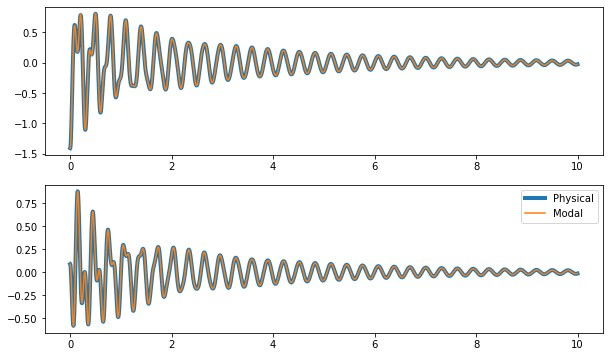
Clearly, the response is not drastically different between the physical and modal models. Therefore, we can consider dropping the off-diagonal terms a reasonable approximation.

Response to Harmonic Excitation

While we can gain significant insight into the system by examining free response, most of the environments that excite structural dynamics involve forces. We will therefore examine the response to harmonic forcing. We will start with the matrix equation, now including damping.

\[\mathbf{M}\ddot{\mathbf{x}}+\mathbf{C}\dot{\mathbf{x}}+\mathbf{K}\mathbf{x} = \mathbf{f}\]

We can substitute the known solution

\[-\omega^2\mathbf{M}\mathbf{X}e^{i\omega t}+i\omega\mathbf{C}\mathbf{X}e^{i\omega t}+\mathbf{K}\mathbf{X}e^{i\omega t} = \mathbf{F}e^{i\omega t}\]

which we can again cancel the transient \(e^{i\omega t}\) due to it being nonzero in general

\[-\omega^2\mathbf{M}\mathbf{X}+i\omega\mathbf{C}\mathbf{X}+\mathbf{K}\mathbf{X} = \mathbf{F}\]

At this point, we will perform the modal transformation by substituting \(\mathbf{X} = \Phi\mathbf{Q}\) and pre-multiplying by \(\Phi^T\). Assuming mass-normalized mode shapes,

\[\begin{split}-\omega^2\begin{bmatrix}1 & & \mathbf{0}\\ & 1 & \\\mathbf{0} & & \ddots \end{bmatrix}\mathbf{Q}+i\omega\begin{bmatrix}2\zeta_1\omega_1 & & \mathbf{0}\\ & 2\zeta_2\omega_2 & \\ \mathbf{0} & & \ddots \end{bmatrix}\mathbf{Q}+\begin{bmatrix}\omega_1^2 & & \mathbf{0}\\ & \omega_2^2 & \\ \mathbf{0} & & \ddots \end{bmatrix}\mathbf{Q} = \Phi^T\mathbf{F}\end{split}\]

or more compactly

\[\left(-\omega^2+i\omega\left[^\ddots2\zeta_n\omega_n{}_\ddots\right]+\left[^\ddots\omega_n^2{}_\ddots\right]\right)\mathbf{Q} = \Phi^T\mathbf{F}\]

We now have a dynamic stiffness matrix in terms of modal mass, modal stiffness, and modal damping matrices. Note, however, that because each degree of freedom is uncoupled from the others (the modal dynamic stiffness matrix is diagonal), inverting this modal dynamic stiffness matrix is equivalent to taking the reciprocal of each term.

\[\mathbf{Q} = \left(-\omega^2+i\omega\left[^\ddots2\zeta_n\omega_n{}_\ddots\right]+\left[^\ddots\omega_n^2{}_\ddots\right]\right)^{-1}\Phi^T\mathbf{F}\]

Finally, we can transform back to physical coordinates by using the modal transformation \(\mathbf{X} = \Phi\mathbf{Q}\)

\[\mathbf{X} = \Phi\mathbf{Q} = \Phi\left(-\omega^2+i\omega\left[^\ddots2\zeta_n\omega_n{}_\ddots\right]+\left[^\ddots\omega_n^2{}_\ddots\right]\right)^{-1}\Phi^T\mathbf{F}\]

Noting that the dynamic stiffness matrix is diagonal, we can reduce this product of 3 matrices to instead a summation of terms.

\[\mathbf{X} = \left(\sum_{k=1}^n {\Phi_k{\Phi_k}^T \over -\omega^2+2i\omega\zeta_k\omega_k+\omega_k^2}\right)\mathbf{F}\]

And we can therefore define the frequency response function matrix \(\mathbf{H}\) in terms of modal parameters such that \(\mathbf{X} = \mathbf{H}\mathbf{F}\)

\[\mathbf{H} = \sum_{k=1}^n {\Phi_k{\Phi_k}^T \over -\omega^2+2i\omega\zeta_k\omega_k+\omega_k^2}\]

where \(\Phi_k\) is the \(k\)th mode shape, \(\omega_k\) is the \(k\)th natural frequency, \(\zeta_k\) is the \(k\)th damping factor, \(\omega\) is the frequency of excitation, and \(i\) is the complex number \(i=\sqrt{-1}\). Note that the above is the frequency response function between force and displacement. We could instead write the frequency response function between force and velocity or force and acceleration by multiplying by \(i\omega\) or \(-\omega^2\), respectively.

This expression for the frequency response function is very informative. We can see that the response is due to a summation of contributions from the different modes of the system, which is denoted by the summation symbol. The fact that the mode shape matrix is in the numerator shows that for a given modal response, locations with larger coefficients in the mode shape for that mode will displace larger amounts. We can also see due to the mode shape matrix transposed in the numerator that forces being applied at locations with larger coefficients in the mode shape matrix will excite larger modal response for that mode. Finally, we see that there is an amplification factor due to the terms in the denominator. We see that as \(\omega\) approaches \(\omega_k\), the denominator will grow smaller and the modal response of the \(k\)th mode will grow larger.

Let’s compute this for our example problem.

frequencies = np.linspace(0,10,1001)
omega = (frequencies*2*np.pi)[:,np.newaxis,np.newaxis]

H_per_mode = []
for omega_k,zeta_k,phi_k in zip(shapes.frequency*2*np.pi,shapes.damping,shapes.shape_matrix[...,np.newaxis]):
    H_per_mode.append(phi_k@phi_k.T/(-omega**2+2j*omega*omega_k*zeta_k+omega_k**2))

fig,ax = plt.subplots(2,2,num='Mode Contributions to FRF',figsize=(10,6),sharex=True,sharey=True)
for i in range(2):
    for j in range(2):
        ax[i,j].plot(frequencies,abs(H_per_mode[0][:,i,j]))
        ax[i,j].plot(frequencies,abs(H_per_mode[1][:,i,j]))
        ax[i,j].plot(frequencies,abs(H_per_mode[0][:,i,j]+H_per_mode[1][:,i,j]))
        ax[i,j].set_yscale('log')
        if i == 1:
            ax[i,j].set_xlabel('Frequency (Hz)\n\nForce Input to DOF {:}'.format(j+1))
        if j == 0:
            ax[i,j].set_ylabel('Response at DOF {:}\n\nFRF Magnitude (m/N)'.format(j+1))

ax[-1,-1].legend(['Mode 1 Contribution','Mode 2 Contribution','Sum of Contributions']);
fig.tight_layout()

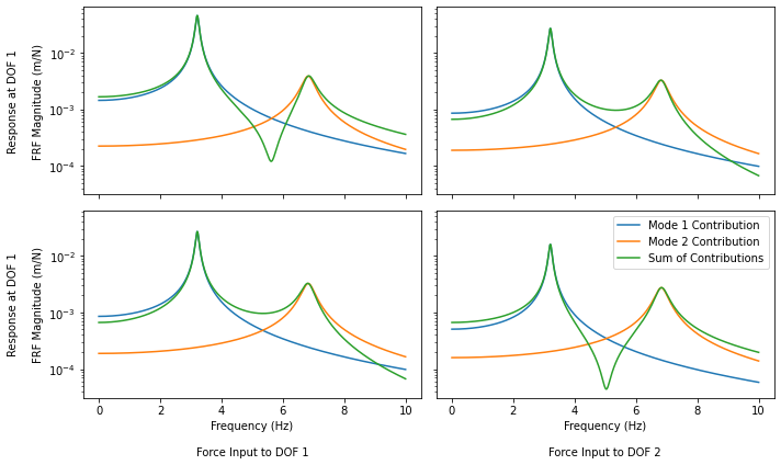
Here you can see the frequency response function matrix for the two degree of freedom system split out into the contributions from each mode. The sum of contributions is also plotted. It may be counterintuitive on the diagonal plots that magnitude of the sum of the two contributions can result in a value that is less than the magnitude of the original two components; however, one must recognize that what is plotted is magnitude of a complex number, and those complex numbers may be out of phase with one another. For an intuitive example, consider the addition of 1 and -1. If we compute the magnitudes, both are equal to 1, but if we sum them together and then compute the magnitude of the summation, we will get zero.

Modal Analysis in SDynPy

Because modal analysis is such a prevalent technique in structural dynamics, it is heavily integrated into SDynPy. Once we have created a System object, we can quickly compute the modes of the system by calling the System.eigensolution() function. To demonstrate, we will use a System from the sdynpy.demo package which contains a plate made of beam finite elements.

from sdynpy.demo.beam_plate import system as plate_system

We will call the eigensolution method of the plate_system to compute the frequencies and mode shapes. Note that if damping were defined in the system, it would also be reduced to modal damping as described previously, and represented by a fraction of critical damping. However, rather than simply returning an array of eigenvalues and a matrix of mode shapes, SDynPy will package them nicely into a ShapeArray object, which contains the mode shapes, the frequencies converted to hertz, the damping ratios, and some comments that can be used to store other metadata. Note that there are various arguments to the eigensolution method that can be used to specify which modes to solve for; for example, we can specify a number of modes to find, or we can specify a maximum frequency up to which modes will be computed.

# Solve for modes above 1000 Hz
plate_shapes = plate_system.eigensolution(maximum_frequency=1000)
print('Computed {:} Modes of the plate system'.format(plate_shapes.size))

Computed 29 Modes of the plate system

If we simply type the ShapeArray object into the command window, it will produce a summary table of the modes in the object.

plate_shapes

   Index,  Frequency,    Damping,     # DoFs
    (0,),     0.0000,    0.0000%,        270
    (1,),     0.0000,    0.0000%,        270
    (2,),     0.0002,    0.0000%,        270
    (3,),     0.0002,    0.0000%,        270
    (4,),     0.0002,    0.0000%,        270
    (5,),     0.0002,    0.0000%,        270
    (6,),    67.4788,    0.0000%,        270
    (7,),   102.0777,    0.0000%,        270
    (8,),   185.1884,    0.0000%,        270
    (9,),   214.7808,    0.0000%,        270
   (10,),   232.2875,    0.0000%,        270
   (11,),   311.9626,    0.0000%,        270
   (12,),   355.5867,    0.0000%,        270
   (13,),   361.3963,    0.0000%,        270
   (14,),   364.7936,    0.0000%,        270
   (15,),   370.0250,    0.0000%,        270
   (16,),   462.3216,    0.0000%,        270
   (17,),   539.8559,    0.0000%,        270
   (18,),   593.8296,    0.0000%,        270
   (19,),   594.6486,    0.0000%,        270
   (20,),   634.0691,    0.0000%,        270
   (21,),   643.6099,    0.0000%,        270
   (22,),   710.9058,    0.0000%,        270
   (23,),   746.4506,    0.0000%,        270
   (24,),   776.8982,    0.0000%,        270
   (25,),   809.6974,    0.0000%,        270
   (26,),   853.9038,    0.0000%,        270
   (27,),   857.0849,    0.0000%,        270
   (28,),   879.0950,    0.0000%,        270

We can access the underlying data using the various attributes of the ShapeArray object.

plate_shapes.frequency

array([0.00000000e+00, 0.00000000e+00, 1.68587394e-04, 1.68587394e-04,
       1.68587394e-04, 1.68587394e-04, 6.74788054e+01, 1.02077709e+02,
       1.85188450e+02, 2.14780834e+02, 2.32287546e+02, 3.11962560e+02,
       3.55586672e+02, 3.61396270e+02, 3.64793564e+02, 3.70025026e+02,
       4.62321608e+02, 5.39855912e+02, 5.93829573e+02, 5.94648580e+02,
       6.34069147e+02, 6.43609950e+02, 7.10905806e+02, 7.46450634e+02,
       7.76898214e+02, 8.09697367e+02, 8.53903834e+02, 8.57084918e+02,
       8.79095024e+02])

plate_shapes.damping

array([0., 0., 0., 0., 0., 0., 0., 0., 0., 0., 0., 0., 0., 0., 0., 0., 0.,
       0., 0., 0., 0., 0., 0., 0., 0., 0., 0., 0., 0.])

print('Shape Matrix Shape {:}'.format(plate_shapes.shape_matrix.shape))
plate_shapes.shape_matrix

Shape Matrix Shape (29, 270)

array([[ 2.87845506e-01, -4.09847824e-01,  2.26589551e-01, ...,
         1.38717885e-01,  4.19171311e-01,  6.29348485e-01],
       [ 1.16437174e-02, -2.74485641e-01, -7.44773478e-02, ...,
        -7.90028325e-01, -6.69589392e-01,  3.67067932e-01],
       [ 1.14736558e-01,  7.97525145e-03, -1.14529355e-01, ...,
        -4.18747047e-01, -2.21629035e-01, -3.16191482e-01],
       ...,
       [ 1.48712418e-15, -3.68911588e-15, -7.12167411e-01, ...,
        -4.07189408e+00,  5.29814800e+00, -3.82376881e-14],
       [-8.23884395e-16, -2.25809218e-14,  5.09546603e-01, ...,
        -9.85048039e+00, -3.35203567e-01, -8.70009100e-14],
       [ 3.29780204e-16, -1.19001068e-14, -2.19373036e-01, ...,
         8.01245326e-01,  7.55525400e+00, -4.88140699e-15]])

Note that the mode shape matrix is stored with the degree of freedom on the last axis of the array, which is transposed compared to the description of the matrix above (for example, the shape of the matrix is 29 modes by 270 degrees of freedom, whereas the \(\Phi\) matrix shown previously would have had a shape of 270 degrees of freedom by 29 modes). This is due to how NumPy stores its data in structured arrays, so the user must be aware that they may need to transpose their array prior to using it calculations. Alternatively, users can access the traditional mode shape matrix with the modeshape property, which returns the shape matrix with its last two dimensions swapped.

print('Modeshape Shape {:}'.format(plate_shapes.modeshape.shape))
plate_shapes.modeshape

Modeshape Shape (270, 29)

array([[ 2.87845506e-01,  1.16437174e-02,  1.14736558e-01, ...,
         1.48712418e-15, -8.23884395e-16,  3.29780204e-16],
       [-4.09847824e-01, -2.74485641e-01,  7.97525145e-03, ...,
        -3.68911588e-15, -2.25809218e-14, -1.19001068e-14],
       [ 2.26589551e-01, -7.44773478e-02, -1.14529355e-01, ...,
        -7.12167411e-01,  5.09546603e-01, -2.19373036e-01],
       ...,
       [ 1.38717885e-01, -7.90028325e-01, -4.18747047e-01, ...,
        -4.07189408e+00, -9.85048039e+00,  8.01245326e-01],
       [ 4.19171311e-01, -6.69589392e-01, -2.21629035e-01, ...,
         5.29814800e+00, -3.35203567e-01,  7.55525400e+00],
       [ 6.29348485e-01,  3.67067932e-01, -3.16191482e-01, ...,
        -3.82376881e-14, -8.70009100e-14, -4.88140699e-15]])

We can easily verify that the mode shapes diagonalize the system. For example we can compare the structure of the mass and stiffnesss matrices, which will show all of the interconnections between degrees of freedom, to the modal mass and stiffness matrices computed by \(\Phi^T \mathbf{M} \Phi\) and \(\Phi^T\mathbf{K}\Phi\) to see that indeed the matrices are diagonalized.

fig,ax = plt.subplots(2,2,num='Matrix Diagonalization',figsize=(10,10),sharex='col')
ax[0,0].spy(plate_system.M,1e-6)
ax[1,0].spy(plate_system.K,1e-6)
ax[0,0].set_title('Physical Matrices')
ax[0,1].spy(plate_shapes.modeshape.T@plate_system.M@plate_shapes.modeshape,1e-6)
ax[1,1].spy(plate_shapes.modeshape.T@plate_system.K@plate_shapes.modeshape,1e-6)
ax[0,1].set_title('Modal Matrices')
ax[0,0].set_ylabel('Mass Matrix')
ax[1,0].set_ylabel('Stiffness Matrix')
fig.tight_layout()

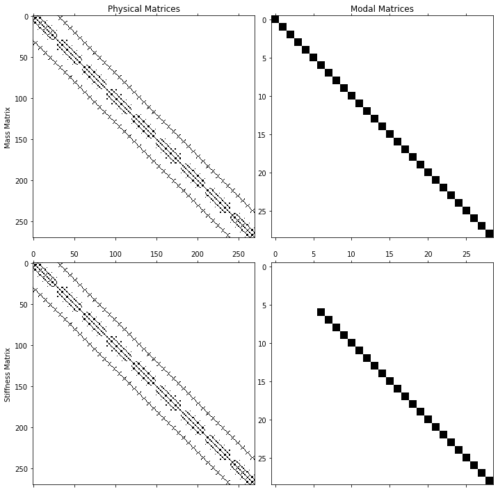
Clearly the physical matrices have some structured coupling between physical degrees of freedom due to the interconnected elements in the model. When we transform into the modal space, we see that the system is diagonalized. Note that because we have not solved for all of the modes in the eigensolution, the number of degrees of freedom in the modal matrices are smaller than the number of physical degrees of freedom, with one for each mode solved. One may also note that the first six entries in the modal stiffness matrix are also missing. These correspond to the rigid body motions of the structure, and there is no stiffness associated with these modes. This can be rationalized by imaginging the system floating out in space with no forces acting on it. If we pushed the structure away from us, which excites its rigid body mode, it will continue floating away indefinitely as there is no restoring force pulling it back. Similarly if we spin it about its axis, it will continue to spin as there is no restoring force to force it to start spinning the opposite direction. Rigid body modes such as this correspond to eigenvalues of zero, and therefore natural frequencies of 0 Hz.

While we could manually set up the modal form of the system by pre- and post-multiplying the mass, stiffness, and damping matrices by the mode shape matrices, SDynPy offers another approach to creating a modal system. The ShapeArray object has a system method that creates a System with modal mass, stiffness, and damping matrices. It also stores the mode shape matrix to use as the transformation between the modal degrees of freedom \(\mathbf{q}\) and the physical degrees of freedom \(\mathbf{x}\).

modal_system = plate_shapes.system()
modal_system

System with 270 DoFs (29 internal DoFs)

We can see the system is built with 29 internal degrees of freedom (these are the modal degrees of freedom) that get transformed via the mode shape matrix to 270 physical degrees of freedom.

Let’s discuss mode shape matrices a bit more. We saw that the mode shape matrix for our system had 270 degrees of freedom for 29 modes. This is a lot of data. While we can look at the values in the matrix directly, and perform math with them, we don’t get a good, intuitive view of what the shapes mean this way. Because the mode shapes represent a deflection shape that the system undergoes as it is vibrating, it would be better if we could visualize this shape as if it were actually the part vibrating. For this we need a few more pieces of information. First, we need a representation of the geometry of the part. We need to know where a point that is vibrating is located, and which direction it should move during the vibration. For this, SDynPy provides a Geometry object. We can get the geometry from the same sdynpy.demo package. We can query the information in the geometry file by typing it into the command window.

from sdynpy.demo.beam_plate import geometry as plate_geometry
plate_geometry

Node
   Index,     ID,        X,        Y,        Z, DefCS, DisCS
    (0,),      1,    0.000,    0.000,    0.000,     1,     1
    (1,),      2,    0.000,    0.125,    0.000,     1,     1
    (2,),      3,    0.000,    0.250,    0.000,     1,     1
    (3,),      4,    0.000,    0.375,    0.000,     1,     1
    (4,),      5,    0.000,    0.500,    0.000,     1,     1
    (5,),      6,    0.125,    0.000,    0.000,     1,     1
    (6,),      7,    0.125,    0.125,    0.000,     1,     1
    (7,),      8,    0.125,    0.250,    0.000,     1,     1
    (8,),      9,    0.125,    0.375,    0.000,     1,     1
    (9,),     10,    0.125,    0.500,    0.000,     1,     1
   (10,),     11,    0.250,    0.000,    0.000,     1,     1
   (11,),     12,    0.250,    0.125,    0.000,     1,     1
   (12,),     13,    0.250,    0.250,    0.000,     1,     1
   (13,),     14,    0.250,    0.375,    0.000,     1,     1
   (14,),     15,    0.250,    0.500,    0.000,     1,     1
   (15,),     16,    0.375,    0.000,    0.000,     1,     1
   (16,),     17,    0.375,    0.125,    0.000,     1,     1
   (17,),     18,    0.375,    0.250,    0.000,     1,     1
   (18,),     19,    0.375,    0.375,    0.000,     1,     1
   (19,),     20,    0.375,    0.500,    0.000,     1,     1
   (20,),     21,    0.500,    0.000,    0.000,     1,     1
   (21,),     22,    0.500,    0.125,    0.000,     1,     1
   (22,),     23,    0.500,    0.250,    0.000,     1,     1
   (23,),     24,    0.500,    0.375,    0.000,     1,     1
   (24,),     25,    0.500,    0.500,    0.000,     1,     1
   (25,),     26,    0.625,    0.000,    0.000,     1,     1
   (26,),     27,    0.625,    0.125,    0.000,     1,     1
   (27,),     28,    0.625,    0.250,    0.000,     1,     1
   (28,),     29,    0.625,    0.375,    0.000,     1,     1
   (29,),     30,    0.625,    0.500,    0.000,     1,     1
   (30,),     31,    0.750,    0.000,    0.000,     1,     1
   (31,),     32,    0.750,    0.125,    0.000,     1,     1
   (32,),     33,    0.750,    0.250,    0.000,     1,     1
   (33,),     34,    0.750,    0.375,    0.000,     1,     1
   (34,),     35,    0.750,    0.500,    0.000,     1,     1
   (35,),     36,    0.875,    0.000,    0.000,     1,     1
   (36,),     37,    0.875,    0.125,    0.000,     1,     1
   (37,),     38,    0.875,    0.250,    0.000,     1,     1
   (38,),     39,    0.875,    0.375,    0.000,     1,     1
   (39,),     40,    0.875,    0.500,    0.000,     1,     1
   (40,),     41,    1.000,    0.000,    0.000,     1,     1
   (41,),     42,    1.000,    0.125,    0.000,     1,     1
   (42,),     43,    1.000,    0.250,    0.000,     1,     1
   (43,),     44,    1.000,    0.375,    0.000,     1,     1
   (44,),     45,    1.000,    0.500,    0.000,     1,     1

Coordinate_system
   Index,     ID,                 Name, Color,       Type
    (0,),      1,                     ,     1,  Cartesian

Traceline
   Index,     ID,          Description, Color, # Nodes
    (0,),      1,                     ,     1,       2
    (1,),      2,                     ,     1,       2
    (2,),      3,                     ,     1,       2
    (3,),      4,                     ,     1,       2
    (4,),      5,                     ,     1,       2
    (5,),      6,                     ,     1,       2
    (6,),      7,                     ,     1,       2
    (7,),      8,                     ,     1,       2
    (8,),      9,                     ,     1,       2
    (9,),     10,                     ,     1,       2
   (10,),     11,                     ,     1,       2
   (11,),     12,                     ,     1,       2
   (12,),     13,                     ,     1,       2
   (13,),     14,                     ,     1,       2
   (14,),     15,                     ,     1,       2
   (15,),     16,                     ,     1,       2
   (16,),     17,                     ,     1,       2
   (17,),     18,                     ,     1,       2
   (18,),     19,                     ,     1,       2
   (19,),     20,                     ,     1,       2
   (20,),     21,                     ,     1,       2
   (21,),     22,                     ,     1,       2
   (22,),     23,                     ,     1,       2
   (23,),     24,                     ,     1,       2
   (24,),     25,                     ,     1,       2
   (25,),     26,                     ,     1,       2
   (26,),     27,                     ,     1,       2
   (27,),     28,                     ,     1,       2
   (28,),     29,                     ,     1,       2
   (29,),     30,                     ,     1,       2
   (30,),     31,                     ,     1,       2
   (31,),     32,                     ,     1,       2
   (32,),     33,                     ,     1,       2
   (33,),     34,                     ,     1,       2
   (34,),     35,                     ,     1,       2
   (35,),     36,                     ,     1,       2
   (36,),     37,                     ,     1,       2
   (37,),     38,                     ,     1,       2
   (38,),     39,                     ,     1,       2
   (39,),     40,                     ,     1,       2
   (40,),     41,                     ,     1,       2
   (41,),     42,                     ,     1,       2
   (42,),     43,                     ,     1,       2
   (43,),     44,                     ,     1,       2
   (44,),     45,                     ,     1,       2
   (45,),     46,                     ,     1,       2
   (46,),     47,                     ,     1,       2
   (47,),     48,                     ,     1,       2
   (48,),     49,                     ,     1,       2
   (49,),     50,                     ,     1,       2
   (50,),     51,                     ,     1,       2
   (51,),     52,                     ,     1,       2
   (52,),     53,                     ,     1,       2
   (53,),     54,                     ,     1,       2
   (54,),     55,                     ,     1,       2
   (55,),     56,                     ,     1,       2
   (56,),     57,                     ,     1,       2
   (57,),     58,                     ,     1,       2
   (58,),     59,                     ,     1,       2
   (59,),     60,                     ,     1,       2
   (60,),     61,                     ,     1,       2
   (61,),     62,                     ,     1,       2
   (62,),     63,                     ,     1,       2
   (63,),     64,                     ,     1,       2
   (64,),     65,                     ,     1,       2
   (65,),     66,                     ,     1,       2
   (66,),     67,                     ,     1,       2
   (67,),     68,                     ,     1,       2
   (68,),     69,                     ,     1,       2
   (69,),     70,                     ,     1,       2
   (70,),     71,                     ,     1,       2
   (71,),     72,                     ,     1,       2
   (72,),     73,                     ,     1,       2
   (73,),     74,                     ,     1,       2
   (74,),     75,                     ,     1,       2
   (75,),     76,                     ,     1,       2

Element
   Index,     ID, Type, Color, # Nodes
----------- Empty -------------

We can see from this information that the geometry consists of four main parts. These are Nodes, Coordinate Systems, Tracelines, and Elements. Nodes represent positions in space. They have a 3D coordinate which locates the point in space. They also have assigned to them a Definition Coordinate System (DefCS) and a Displacement Coordinate System (DisCS). These identify which coordinate system the coordinate points are defined, and which coordinate systems the displacements occur. Nodes can be referenced by the Geometry.node attribute, and consist of a NodeArray object.

The identifiers for the coordinate systems reference IDs in the Coordinate System portion of the geometry. The current geometry only has a single coordinate system that represents the global coordinate system. However, different geometries might have additional local coordinate systems, which could even be cylindrical or spherical coordinate systems. Coordinate systems can be referenced by the Geometry.coordinate_system attribute, and consist of a CoordinateSystemArray object.

Finally, it can be hard to visualize a geometry just looking at points in space, so the geometry defines Elements and Tracelines, which are used to connect the node positions to make visualization easier. Tracelines can be referenced by the Geometry.traceline attribute and consist of a TracelineArray object. Elements can be referenced by the Geometry.element attribute and consist of a ElementArray object.

Once again, it can be difficult to visualize the geometry just by looking at the values of the coordinates, so SDynPy provides the ability to plot the geometry in an interactive window. This is done by calling the Geometry.plot method. Various arguments can be given to this method to determine how the plotting should be performed.

plate_geometry.plot();

Here we see the plate geometry rotating in the figure. By clicking and dragging the mouse in the plot window, the view of the geometry can be rotated to a preferrable view. Using the mouse scroll wheel will zoom the plot in and out. Clicking and dragging with the middle mouse button will pan the view.

So we have geometry, and we have our mode shapes, but how do the values in the mode shapes get mapped to deflections on the geometry? How do we know which row in our mode shape matrix corresponds to which node of our geometry? To perform this mapping, a CoordinateArray is used. A CoordinateArray objects consists of a node ID number and a direction (e.g. 101X+, which would mean node 101 will move in the positive \(x\) direction in the geometry). If we look closer at our mode shape objects, we can see that they actually have a coordinate attribute defined that contains a coordinate array. This coordinate array is the same shape as the shape matrix data, and defines how each entry in the mode shape maps to a position and direction on the geometry.

print('The shape matrix has shape {:} and the coordinate has shape {:}'.format(
    plate_shapes.shape_matrix.shape,plate_shapes.coordinate.shape))
plate_shapes.coordinate

The shape matrix has shape (29, 270) and the coordinate has shape (29, 270)

coordinate_array(string_array=
array([['1X+', '1Y+', '1Z+', ..., '45RX+', '45RY+', '45RZ+'],
       ['1X+', '1Y+', '1Z+', ..., '45RX+', '45RY+', '45RZ+'],
       ['1X+', '1Y+', '1Z+', ..., '45RX+', '45RY+', '45RZ+'],
       ...,
       ['1X+', '1Y+', '1Z+', ..., '45RX+', '45RY+', '45RZ+'],
       ['1X+', '1Y+', '1Z+', ..., '45RX+', '45RY+', '45RZ+'],
       ['1X+', '1Y+', '1Z+', ..., '45RX+', '45RY+', '45RZ+']], dtype='<U5'))

We can see that not only are there translational coordinates in our mode shape matrix (X+,Y+,Z+), but there are also rotational degrees of freedom in our shape matrix (RX+,RY+,RZ+) which correspond to rotations about the \(x\), \(y\), and \(z\) directions, respectively. We can see how those degrees of freedom map to the geometry by plotting them using the Geometry.plot_coordinate method.

plotter = plate_geometry.plot_coordinate(
    np.unique(plate_shapes.coordinate), # Use np.unique to remove duplicate coordinates
    arrow_scale=0.025,label_dofs = True)

As you can see, the degrees of freedom are now shown on the geometry and labeled so the user can identify them. So, for example, if a mode shape has a coordinate of 1X+ and a coefficient of 0.5, it means that node 1 in the geometry will be translated 0.5 units in the positive \(x\) direction.

So now that we’ve determined how the mode shapes get mapped to the geometry, let’s try plotting a mode shape on the geometry. This is done with the Geometry.plot_shape method. This will bring up a window with the mode shape overlaid on the geometry.

plate_geometry.plot_shape(plate_shapes);

The animation of the shape can be controlled using the toolbar at the top of the window. Pressing Start or Stop will start or stop the animation. Pressing << or >> will proceed to the previous or next shape. There are more options in the Shape menu at the top of the window to control the speed of the animation or the scale of the animation. Animations can be saved to .gif files via the File Menu.

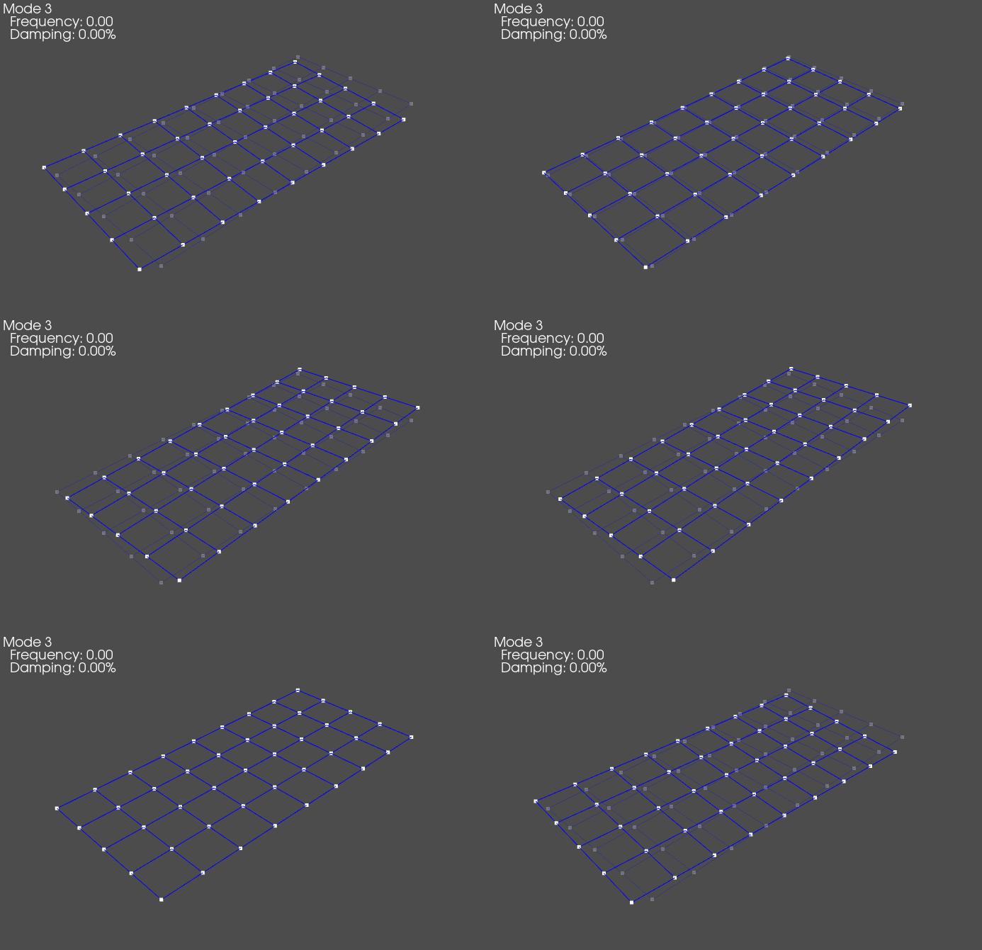
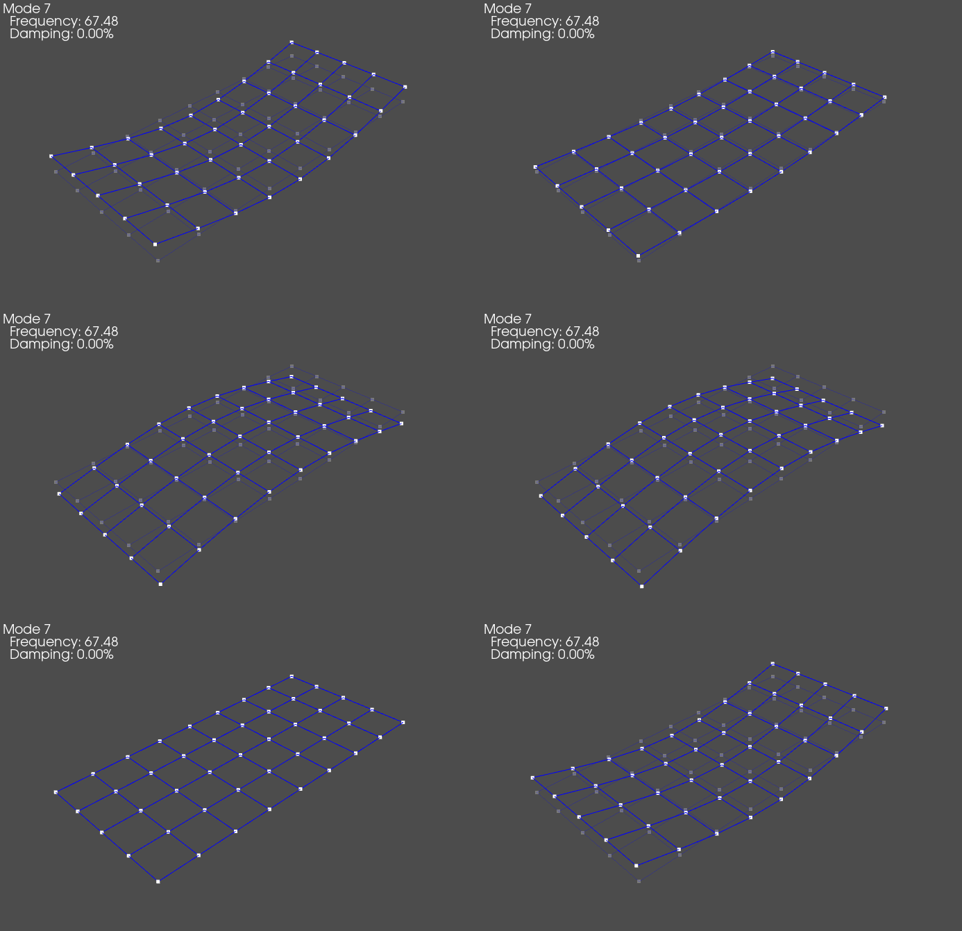
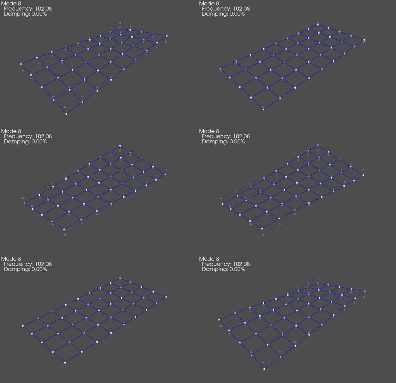
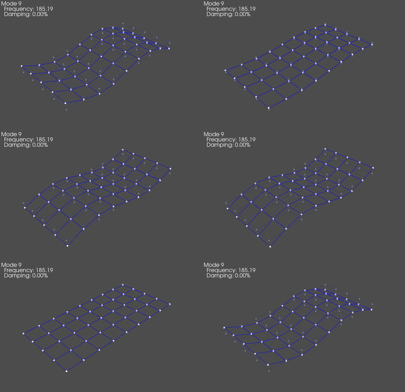
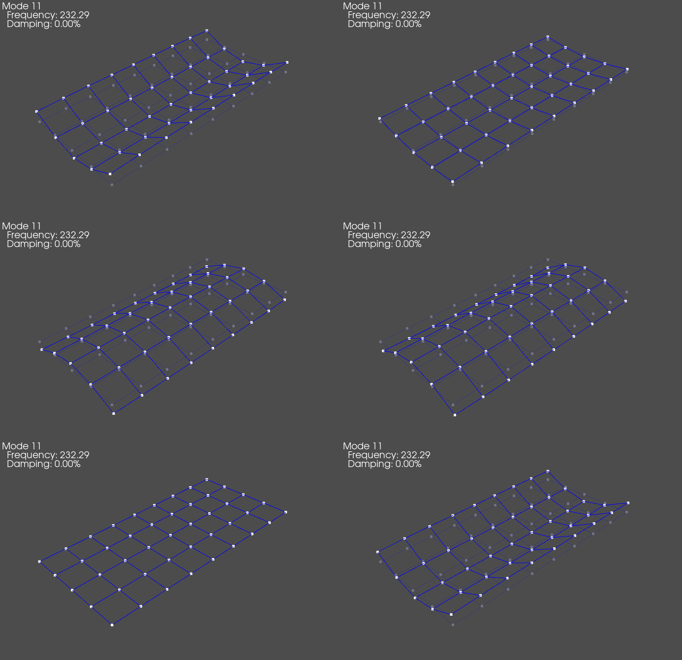
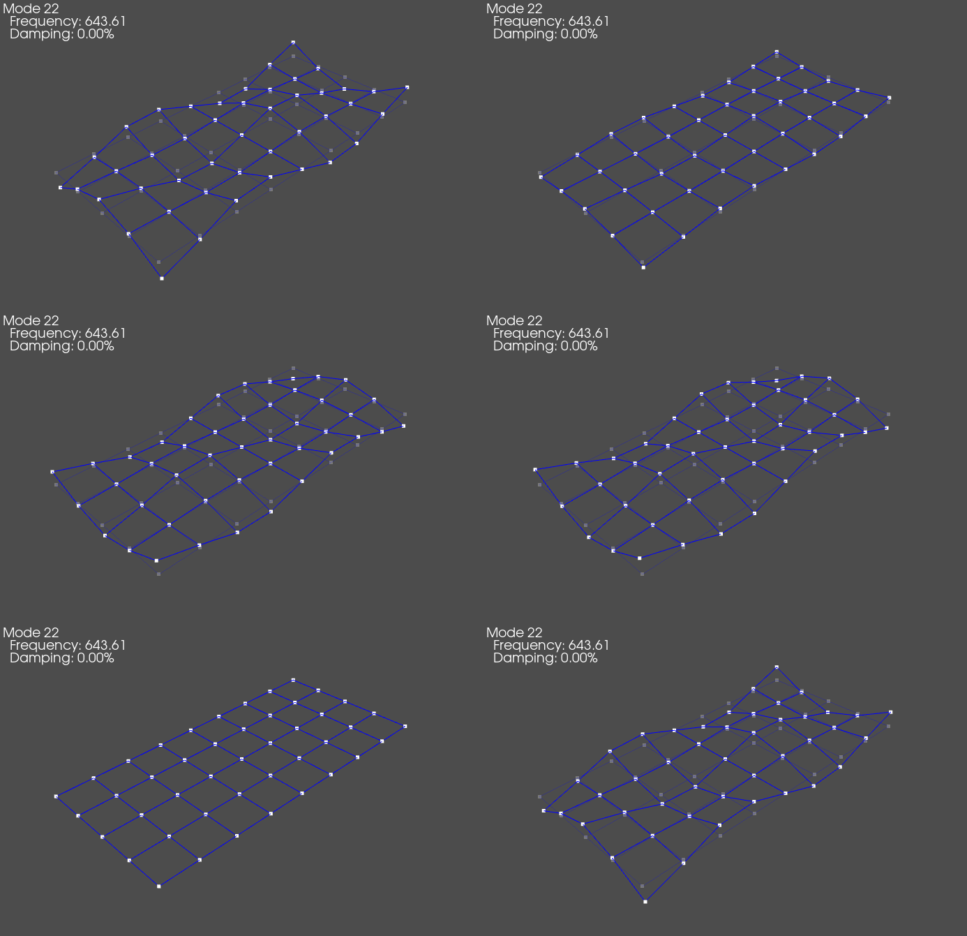
Note that the 0 Hz modes will generally have a rigid looking response, i.e. only a translation or rotation, no bending. The plate then has various classes of shapes, and different orders of those shapes. For example, shown above are a rigid body shape, a bending about the long direction of the plate, a twisting or torsion of the plate, a second bending about the long direction of the plate, a bending about the short direction of the plate, and finally a higher-order mode that is difficult to describe. Generally, as the shapes get higher in frequency, they become more complex, though there can be exceptions (for example, the first bending in the short direction comes after the second bending in the long direction in this case, due to the geometry of the part).

It should be clear that visualizing the shapes by deforming the geometry gives a much more intuitive view of the mode shape than simply examining the values in the mode shape matrix.

Summary

This tutorial has introduce Modal Analysis, which is the process of transforming a potentially complex system into a set of much simpler single-degree of freedom systems, which can be analyzed much more easily. We identified how the modes of a system derive from the non-trivial solutions to the free response of systems of equations. We solved for the natural frequencies and mode shapes of a system by solving the generalized eigenvalue problem, where the eigenvalue was equal to the angular natural frequency squared, and the eigenvector was equal to the mode shape. We then saw how we could perform those same operations in the SDynPy framework, including how to plot mode shapes on the system’s geometry for a more intuitive view of what the deformations in each shape look like.

The next tutorial will introduce Experimental Modal Analysis, which will be the process by which modes can be identified in real systems without knowing the mass and stiffness matrices of the system.

Homework Problems

1. Construct the generalized eigenvalue problem

Using the homework problem from the previous tutorial, write equation for the eigenvalue problem using the mass and stiffness matrices.

\(m_1=10\), \(m_2 = 30\), \(m_3 = 1\), \(k_1 = 10000\), \(k_2 = 2500\), \(k_3 = 1500\), \(k_4 = 1500\), \(c_1 = 30\), and \(c_2 = 50\).

2. Compute and solve the characteristic polynomial

Compute the characteristic polynomial via the determinant of the eigenvalue problem from the previous problem. Solve the polynomial for the eigenvalue \(\lambda\) and then convert to angular frequency \(\omega\) in radians per second and frequency in hertz. How many eigenvalues did you compute, and how many should there be given the number of degrees of freedom of the system?

3. Compute eigenvector

Compute the eigenvector for the lowest natural frequency computed in the previous problem. Use the approach where one of the values is set to 1 and the remaining values are solved for. After the full vector is computed, compute the mass normalized version of the mode shape such that \(\Phi^T\mathbf{M}\Phi=1\)

4. Perform the same operations in SDynPy and plot the mode shapes

Create a geometry with 3 nodes, with node 1 at (0,0,0) corresponding to mass \(m_1\), node 3 at (1,-0.5,0) corresponding to mass \(m_3\), and node 2 at (2,0,0) corresponding to mass \(m_2\). Connect the three masses with tracelines if you would like. Construct a system with mass, stiffness, and damping matrices given the values in Problem 1. Set the coordinates to 1X+, 2X+ and 3X+ so the displacements in the mode shapes are in the positive \(x\) direction for each node. Solve the eigensolution and plot the mode shapes on the geometry.

5. Compute the FRF matrix from modal quantities

Compute the FRF matrix from the modal quantities computed in Problem 4. Compare it to the FRF matrix from Problem 2 in the previous tutorial.