Analysis of Transient Finite Element Results

One use-case of SDynPy could be for analyzing transient data from finite element analysis. While many structural dynamics codes will, for instance, automatically compute eigensolutions to compute the modes of the system, we must sometimes use transient solutions to analyze systems. For example, if there is contact or other nonlinearities that we wish to account for, then we can’t in general use a linear finite element code to perform that solution. This example will demonstrate how to use SDynPy to perform modal analysis on the results of a transient solution from Sierra/SolidMechanics’s explicit solver.

Contents

• Analysis of Transient Finite Element Results

  • Problem Set Up

  • Analyzing Model Responses

    • Pseudorandom Analysis

    • Random Analysis

  • Comparison of Excitation Techniques

  • Summary

Problem Set Up

The problem we are investigating here is a simple cantilevered fork structure.

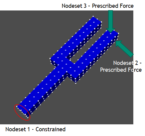
Tuning fork setup

We will constrain the base of the fork using a fixed displacement boundary condition at nodeset 1, and nodeset 2 and 3 are defined such that external forces may be applied. The frequency range of interest for this analysis will be up to 2000 Hz.

If the goal is to characterize the model rather than, for example, simulate an environment, it can be useful to apply standard forcing signals to the part, essentially performing a simulated modal test on the structure. In this example, we will investigate single-input excitation using Pseudorandom excitation and multiple-input excitation using Random excitation. Both of these signals can be generated by SDynPy’s sdpy.generator module.

The first step will be to import the required packages

import sdynpy as sdpy           # For structural dynamics operations
import numpy as np              # For numeric operations
import matplotlib.pyplot as plt # For plotting

Then we will generate signals using the sdpy.generator module. First, we will generate the Pseudorandom signal, using the sdpy.generator.pseudorandom function.

We will generate the signal such that each frame of data is 1 second long, meaning the number of frequency lines is equal to the Nyquist frequency of 2000 Hz. This results in a 1 Hz frequency spacing, which is equivalent to a 1 second measurement frame. The signal will be generated such that is has a level of 1 N RMS, and we will truncate the signal at 5 Hz, because frequencies below that are not interesting in this analysis. We specify 10 averages, and an integration_oversample of 10. This last parameter ensures that the linear interpolation performed by Sierra/SolidMechanics results in a smooth sine wave even at the Nyquist frequency of the analysis.

# Generate the pseudorandom signal
times,pseudorandom_signal = sdpy.generator.pseudorandom(
    fft_lines = 2000, f_nyq = 2000, signal_rms = 1, min_freq = 5,
    integration_oversample=10, averages=10)

This signal is quite long, so it would be very clumbsy to write this directly into the input file for the analysis. This would result in a large amount of scrolling to get to other portions of the input file. Instead, we will write the signal to another file, which will be included in the main input file for the analysis.

with open('pseudorandom_signal.inc','w') as f:
    for t,s in zip(times,pseudorandom_signal):
        f.write('{:} {:}\n'.format(t,s))

We can then plot the signal and its FFT to verify that it is constructed correctly.

# Compute the FFT and frequency bins
freq = np.fft.rfftfreq(
    pseudorandom_signal.shape[-1],
    np.mean(np.diff(times)))
pseudorandom_signal_fft = np.fft.rfft(pseudorandom_signal)

# Plot them
fig,ax = plt.subplots(2,1,num='Pseudorandom Signal')
ax[0].plot(times,pseudorandom_signal)
ax[1].plot(freq,np.abs(pseudorandom_signal_fft))
ax[0].set_ylabel('Force (N)')
ax[1].set_ylabel('FFT Force (N)')
ax[0].set_xlabel('Time (s)')
ax[1].set_xlabel('Frequency (Hz)')
ax[0].set_title('Pseudorandom Excitation')
fig.tight_layout()

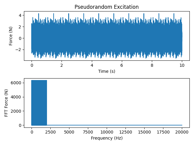
Pseudorandom signal applied to the tuning fork

We can see that the signal repeats 10 times, once for each average specified. We can also see that the frequency content ends abruptly at 2000 Hz, which is the Nyquist frequency specified. However, due to the integration oversampling, the FFT is zero-padded up to 10 times the Nyquist frequency.

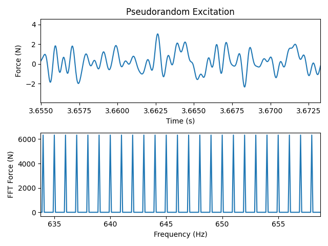
Zoomed in portion of the pseudorandom signal

Zooming in on the signal, we can see more information. We see that the signal is indeed smooth, due to the oversampling specified. There are no sharp features in the signal. Additionally, we can see that only every 10th frequency bin has content. This is due to the averaging, which increases the signal length and therefore decreases the frequency bin spacing of the FFT. However, because we will be averaging the signals together and therefore shortening the signal during the signal processing that will occur, we will lose these intermediate frequency bins, and any content that is in them will result in spectral leakage. It is therefore correct that these frequency bins should have zero frequency content.

We can do similar for the random signal that we wish to generate, using the sdpy.generator.random function. Again, we will generate the signal such that it is 1 second long to achieve 1 Hz frequency spacing. We will generate two independent signals, to excite the structure simultaneously from two different directions. Because random is not a deterministic signal, we will need to specify more averages than in the pseudorandom case, so we specify 30 here. We will again oversample by 10 times to ensure the signal can be smoothly interpolated. Here we must also specify a high_frequency_cutoff to ensure that when we downsample the random data, there is no frequency content past the Nyquist frequency.

# Generate the random signal
dt = 1/4000
signal_shape = (2,)
averages = 30
samples_per_frame = 4000
oversample = 10

random_signal = sdpy.generator.random(
    signal_shape,samples_per_frame*averages*oversample,rms = 1.0,
    dt = dt/oversample, high_frequency_cutoff = 2000)

times = dt/oversample*np.arange(random_signal.shape[-1])

Again, we will write these even longer signals to a separate file to be included in the input file. We will write each signal to a separate file.

for index,signal in enumerate(random_signal):
    with open('random_signal_{:}.inc'.format(index+1),'w') as f:
        for t,s in zip(times,signal):
            f.write('{:} {:}\n'.format(t,s))

Finally, we will again plot the signal to ensure it is constructed correctly.

# Compute the FFT and frequency bins
freq = np.fft.rfftfreq(
    random_signal.shape[-1],
    np.mean(np.diff(times)))
random_signal_fft = np.fft.rfft(random_signal)

# Plot them
fig,ax = plt.subplots(2,1,num='Random Signal')
ax[0].plot(times,random_signal.T)
ax[1].plot(freq,np.abs(random_signal_fft.T))
ax[0].set_ylabel('Force (N)')
ax[1].set_ylabel('FFT Force (N)')
ax[0].set_xlabel('Time (s)')
ax[1].set_xlabel('Frequency (Hz)')
ax[0].set_title('Random Excitation')
fig.tight_layout()

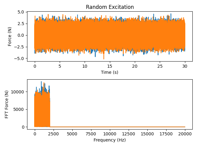
Random signal applied to the tuning fork

We can see now that there is no obvious repetition in the signal. There is also no frequency content past the Nyquist frequency of the test, which is 2000 Hz.

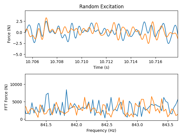
Zoomed in portion of the random signal

Zooming in on the signal, we see that the signal is still smooth due to the oversampling, which is necessary for accurate interpolation. We also see that there is now frequency content in all frequency bins up to the Nyquist. This is due to there not being any repetition in the signal. When we do the signal processing and reduce down to a single frame of data, these frequency bins will result in spectral leakage, so we will need to handle that appropriately by windowing the signal.

With the signals generated, the input deck can be completed. In the function definitions, we include the file that we wrote that contains the forcing function.

begin function pseudorandom
    type = piecewise linear
    begin values
        {include("pseudorandom_signal.inc")}
    end
end function pseudorandom

We can then apply that function to nodesets in the model using the begin prescribed force block.

begin prescribed force
    node set = nodelist_2
    direction = y
    function = pseudorandom
end

Ensure that aprepro processing is used when running Sierra with the -a flag to ensure the included files are processed correctly.

Some other brief notes on setting up the analysis:

1. The termination time is set to the length of the signal to stop the analysis when the signal runs out.

2. Damping is added using proportional damping with mass coefficient 2 and stiffness coefficient 0.0000025.

3. Output is reported every 0.00025 seconds, which corresponds to a 4000 Hz sample rate, which is twice the Nyquist frequency of our signals. If numerical noise is present in the analysis, it may be useful to oversample the output and then apply a filter to remove some of this noise before downsampling.

4. Acceleration and displacement variables were output from the analysis. Either can be analyzed, but we must tell the mode fitter which data type the data is. External forces are also output so we can recover the forcing function to use as reference to the frequency response function.

Analyzing Model Responses

After the models are run, we can load the data in and analyze it as if it were test data. For this example, we will use the Graphical tools in SDynPy to compute frequency response functions and fit modes.

Pseudorandom Analysis

In our pseudorandom analysis code, we will first import the required packages and then load in the Exodus file.

# Import packages
import sdynpy as sdpy
import numpy as np

# Load in the exodus file
exo = sdpy.Exodus('tuning_fork_pseudorandom.e')

Typing the variable name into the console will give us information about what is in the results file.

In [1]: exo
Out[1]:
Exodus File at tuning_fork_pseudorandom.e
  40002 Timesteps
  333 Nodes
  144 Elements
  Blocks: 1
  Node Variables: displacement_x, displacement_y, displacement_z, acceleration_x, acceleration_y, acceleration_z, force_external_x, force_external_y, force_external_z
  Global Variables: external_energy, internal_energy, kinetic_energy, momentum_x, momentum_y, momentum_z, timestep

We can see that the displacement variables are called displacement_x, displacement_y, and displacement_z, and there are also acceleration responses called acceleration_x, acceleration_y, and acceleration_z. External forces are also reported on the model; these are called force_external_x, force_external_y, force_external_z and will contain all forcing applied to the model.

The first thing we will do is create a Geometry object from the Exodus results using its Geometry.from_exodus method.

# Load in the geometry
geometry = sdpy.Geometry.from_exodus(exo)

This will result in a geometry object containing the nodes and element connectivity. We can plot the geometry to ensure it was loaded successfully.

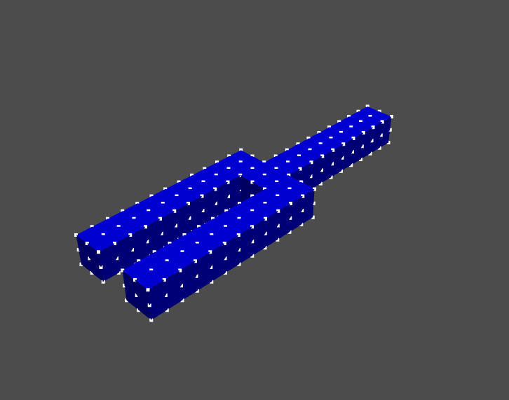
Tuning fork geometry

We can also load in the time data into a TimeHistoryArray using its TimeHistoryArray.from_exodus method. Note that the default arguments to the TimeHistoryArray.from_exodus method assume Sierra/SD variable names DispX, DispY, and DispZ, so we will have to explicitly tell the method which variables to grab. Note that we could grab either acceleration or displacement data this way.

# We could get displacements like this:
response_data = sdpy.TimeHistoryArray.from_exodus(
    exo,'displacement_x','displacement_y','displacement_z')

# Or we can get accelerations like this:
# response_data = sdpy.TimeHistoryArray.from_exodus(
#     exo,'acceleration_x','acceleration_y','acceleration_z')

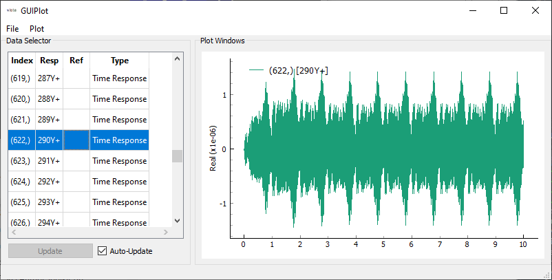
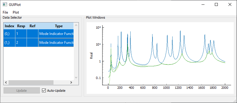
To make sure the data was loaded correctly, we can plot it. This can be done either as 2D data using GUIPlot or as 3D data using the geometry.plot_transient method. For plotting 3D data with long transient signals, it is often better to reduce the size of the data to make the user interface more responsive. We can reduce to only the first second of data using the response_data.extract_elements_by_abscissa method and passing the start abscissa as 0 and the end abscissa as 1.

Note that the displacements will be quite small, so it will be useful to scale the displacements on the 3D animation so they are visible.

# Plot the response data
gui = sdpy.GUIPlot(response_data) # 2D Plot
plotter = geometry.plot_transient(response_data.extract_elements_by_abscissa(0,1)) # 3D Plot

Tuning fork displacement plot using GUIPlot

Tuning fork displacement animation from the geometry.plot_transient function

The last piece of data needed is the force, which will be used as a reference signal to compute frequency response functions. Rather than extracting data using the TimeHistoryArray.from_exodus method, we will instead demonstrate how to interrogate the Exodus file directly and produce a TimeHistoryArray using the sdpy.data_array function.

# Get the node from the nodeset that the force was applied to
force_node = exo.get_node_set_nodes(2)
# Get the y-direction external force applied at that node.
excitation_force_signal = exo.get_node_variable_value('force_external_y',
                                                      force_node[0])
# Set up coordinate information by indexing the node number map.
coord = sdpy.coordinate_array(exo.get_node_num_map()[force_node],2)

# Convert to a TimeHistoryArray
force_data = sdpy.data_array(sdpy.data.FunctionTypes.TIME_RESPONSE,
                             response_data[0].abscissa,
                             excitation_force_signal,
                             coord)

We can then combine our reference signal with the response signals and pass all the data to the sdpy.SignalProcessingGUI. We can assign the geometry to the tool by assigning to the geometry attribute instead of saving it to a file and loading it from graphical user interface.

# Concatenate into a single file
all_data = np.concatenate((force_data[np.newaxis],response_data))

# Analyze the data
gui = sdpy.SignalProcessingGUI(all_data)
gui.geometry = geometry

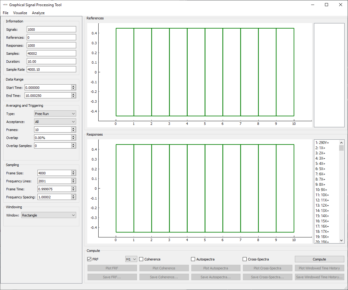
Initial appearance of the SignalProcessingGUI window

Let’s first explore the SignalProcessingGUI Window. On the top left is a set of Information about the signals that are loaded. We see there are 1000 signals total, of which 0 are references and 1000 are responses (we will fix this shortly). There are 40002 samples for a duration of 10 seconds, and the sample rate is 4000.10 Hz (note that there is some uncertainty in when the Exodus file is written to in Sierra/SM, which explains the small divergence from the desired 4000 Hz).

Below the information we have the Data Range. This allows us to select a range over which the computation will be performed. This is useful for targetting portions of an environment, or for discarding portions of data that are not yet at steady state.

Below that are the Averaging and Triggering settings. This allows users to specify when the frames occur in the signal, either by setting them up every so many samples, or detecting some kind of trigger signal to use to locate the measurement frames.

Below that are the Sampling options, where the frame length is specified.

Finally, the last options are for Windowing. Certain windows may have extra parameters that will appear in this box. For example, the decay of an exponential window.

In the center of the window, we see two plots that are currently empty except for some green boxes. These green boxes represent the measurement frames in the signal. Currently no signals are plotted, because we have not selected any signals from the lists on the right side of the window. There are currently no signals listed in the References list; all are currently in the Responses list. Signals can be moved from reference to response and vice versa by double-clicking the signal name in the list on the right side. Note also that when a signal is clicked, it will be shown in the respective plot.

Finally, on the bottom right corner of the window, we have signal processing computations that can be performed. The check boxes denote which functions to compute when the Compute button is pressed. Once a function is computed, it can be plotted or saved to a file.

There are also menus at the top of the window that contain additional functionality. The File menu allows data to be loaded directly from the disk. The Visualize menu allows the data to be sent to the transient or deflection shape plotters once a geometry is loaded (or assigned via code as we have done). The Analyze menu allows data to be sent to curve fitting software, though these are currently disabled until frequency response functions have been computed.

To start with, we will send our force, which is the first signal in the list to the references list by double-clicking it. We should now see that signal as a reference in the top list and plotted in the top plot. Let’s also select the drive point response in the bottom list (only single click, not double click) so it is plotted in the bottom plot.

The first thing we will check is our sampling. We set up our signals to provide 1 Hz frequency spacing, and we can see that the SignalProcessingGUI window has defaulted to the correct frame size to provide that spacing. We therefore do not have to change anything about the frame length. Additionally, with Pseudorandom excitation, we will not need to apply any windows or overlap to the data, so those can stay unchanged as well.

We are nominally exciting the structure with the same excitation for each measurement frame, so the response should be identical for each measurement frame as well. However, we can see that there is some start-up transients that make the first frame not identical to the others, so we would like to discard that first frame. We can change the Acceptance: selector from All to Select and then click on the green rectangle representing the first frame to reject it. The box should turn red when this happens, and the Frames counter should decrease from 10 to 9.

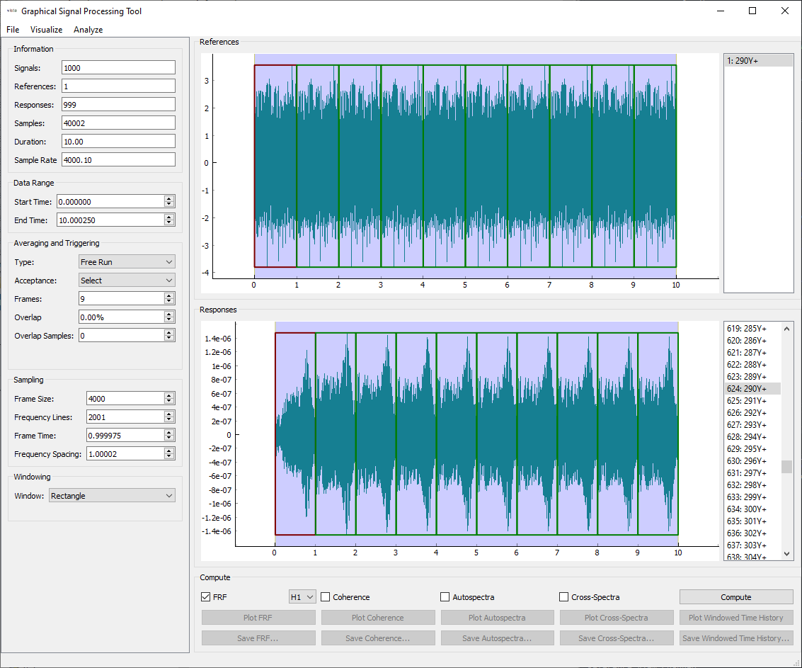
SignalProcessingGUI window after rejecting the first frame

At this point, we will compute the desired functions. We will select the FRF checkbox (keeping H1 as the desired estimator) and also select Coherence. We can then press the Compute button to perform the computations. You should notice that the Plot and Save buttons for the FRF and Coherence have been enabled. We can plot these functions to see if they look correct or not.

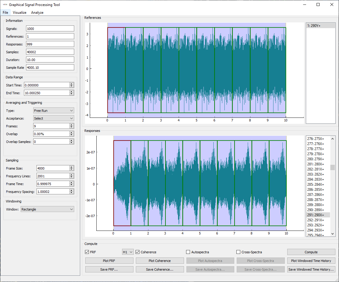
SignalProcessingGUI window after computing the functions

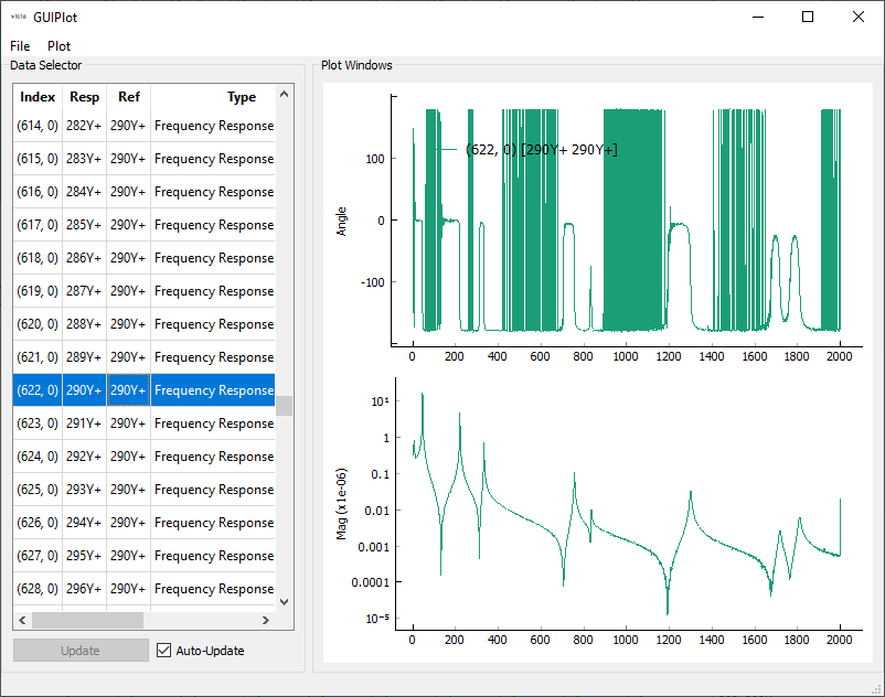
FRF computed from SignalProcessingGUI

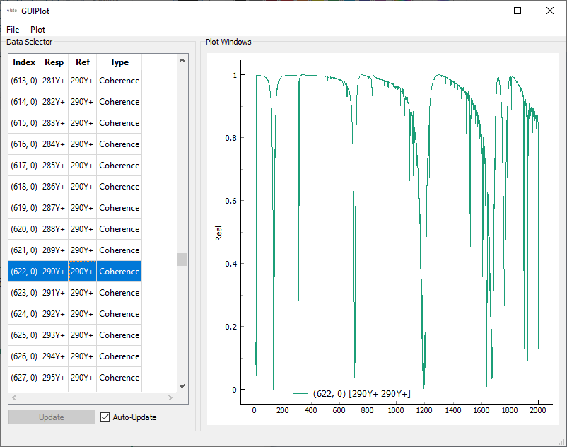
Coherence computed from SignalProcessingGUI

The frequency response functions are clean and the coherence is high at the modes of the structure. We can quickly investigate the different deflection shapes using the Deflection Shape Plotter, which can be accessed via the Visualize menu.

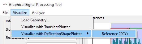
Selecting the deflection shape plotter

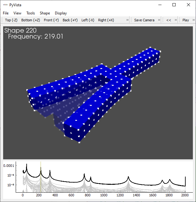
Deflection shape plotter showing the shape at 219 Hz.

To fit modes to the FRFs, we can send the FRFs to a curve fitter via the Analyze menu.

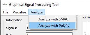
Selecting PolyPy to analyze the FRFs

We will use PolyPy in this example. Selecting Analyze with PolyPy will bring up the PolyPy window with the computed FRFs loaded. PolyPy is a multi-reference Z-domain polynomial curve fitter. The mode fitting process consists of two parts. In the first phase, the roots of the polynomial are solved for a number of different polynomial orders. The roots are generally either real modes of the system or computational roots. The real roots will generally be stable, or occur with the same frequency and damping regardless of the order of the polynomial being solved. The computational roots, on the other hand, will tend to appear spuriously thoughout the frequency range. In the second phase of the curve fitting process, the user will select these stable roots from a stability diagram.

In present PolyPy implementation, the user can select a mode indicator function to plot. The Complex Mode Indicator Function (CMIF) is the singular values of the FRF matrix, and will show peaks where modes are located. The QMIF is a version of the CMIF computed using only the imaginary part of the FRF matrix, and can be more sensitive to modes than the regular CMIF. The Normal Mode Indicator Function (NMIF) and Multi-Mode Indicator Function (MMIF) both denote modes as dips in the indicator function.

In the first phase, the user should also specify the Polynomial Order. These are the orders for which the system will be solved. Generally, the larger the polynomial order, and more orders solved, the longer it will take to create the stability diagram in the second phase of the curve fitter. However, enough orders need to be solved to identify the stability trends. In this case, we will solve between polynomial orders from 20 to 40 by 1, which will solve the system for polynomials orders 20, 21, 22, … , 38, 39, 40.

Users should also specify the type of FRF in the data. The default is set to Acceleration over force FRFs; however, the current FRFs are displacement over force, so the Data Type should be set to Displacement.

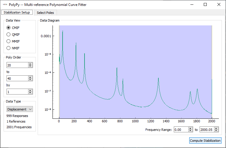
PolyPy setup phase with Poly Order and Data Type set

Once the parameters are set, the Compute Stabilization button can be pressed. The stabilization calculation can take a while depending on the size of the FRF matrix and polynomial orders selected. Status messages will appear in the Python console. When the computation is done, the stability diagram will be shown. In this diagram, the polynomial roots are shown overlaying a mode indicator function to aid in selecting the real roots of the system. Roots of the polynomial will be represented using symbols, depending on the stability achieved. A red X will mean that the root is unstable and shouldn’t be selected. A blue triangle means that the frequency has stabilized, but not the damping or participation factor. A blue square will mean that the frequency and damping have stabilized, and a green circle will mean that the frequency, damping, and participation factors have stabilized. Generally, green circles should be selected, and there are rules of thumb suggesting which green circle to select; for example, many people will generally choose the third or fourth green circle after stabilization occurs. The PolyPy implementation will report the frequency and damping of the root while the mouse is hovering over it to allow the user to understand the stability. Hovered roots will be highlighted black.

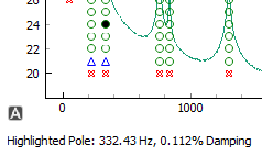
Hovering over a root in PolyPy displays the frequency and damping.

Roots can then be selected by clicking on them. If the Auto-Resynthesize checkbox is checked, PolyPy will immediately compute shapes and resynthesize FRFs after each root selection to allow the user to see the immediate impact of their selection. For large problems, this resynthesis can take a bit of time, so users may wish to deselect this checkbox and simply resynthesize after all roots have been selected. Selected roots will appear colored in, and the frequency, damping, and stability will be reported in the Poles table.

Users can select whether or not to compute complex modes by selecting the Complex Modes checkbox, and they can also specify if residuals should be used to compute the resynthesized FRFs by selecting the Residuals checkbox, which can improve shape accuracy.

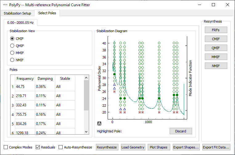
Roots selected for each mode in the stability diagram

Clicking the Resynthesize button will compute mode shapes and resynthesize the FRF matrix so the modal fits can be compared against the experimental data. These shapes can be plotted by first loading in a geometry using the Load Geometry button, and the clicking the Plot Shapes button. Note that the FRFGUI window will automatically pass its geometry to the curve fitter, so we do not need to load a geometry here.

Mode shape for the mode extracted at 332 Hz

Users can judge the adequacy of their fits by clicking one of the buttons in the Resynthesis box on the right side of the window. Individual FRFs can be compared, or data can be accumulated into a mode indicator function and plotted to give an overall view of the fit adequacy.

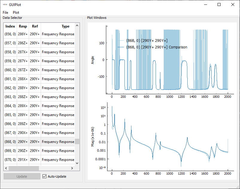
Comparison of initial FRFs to resynthesized FRFs showing good modal fits have been obtained

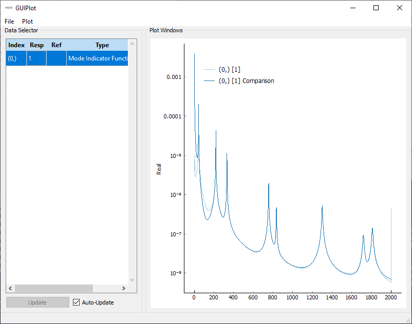
Comparison of initial CMIF to resynthesized CMIF showing good modal fits have been obtained

Users can then export the shapes to a file by clicking the Export Shapes or Export Fit Data buttons. The Export Shapes button only saves the shape data to the disk. The Export Fit Data additionally saves the input FRFs and resynthesized FRFs to the disk, which gives a more complete picture of the fit adequacy. We will save the shape data to disk so we can compare against the shapes obtained from the Random excitation.

Random Analysis

The Random response data will be extracted from the model similarly to the Pseudorandom response data. This time we will read in acceleration data rather than displacement data.

import sdynpy as sdpy
import numpy as np

exo = sdpy.Exodus('tuning_fork_random.e')
geometry = sdpy.Geometry.from_exodus(exo)
# response_data = sdpy.TimeHistoryArray.from_exodus(
#     exo,'displacement_x','displacement_y','displacement_z')
response_data = sdpy.TimeHistoryArray.from_exodus(
    exo,'acceleration_x','acceleration_y','acceleration_z')

In this example, there are two nodes which have forces applied to them, and these correspond to nodesets 2 and 3, with excitation in the \(y\) and \(z\) directions, respectively. We can perform the same operations to extract the forces, except this time we will use a for loop to loop over each signal.

force_data = []
for nodeset,direction in zip([2,3],['y','z']):
    force_node = exo.get_node_set_nodes(nodeset)
    excitation_force_signal = exo.get_node_variable_value('force_external_'+direction,force_node[0])
    force_data.append(sdpy.data_array(sdpy.data.FunctionTypes.TIME_RESPONSE,response_data[0].abscissa,
                                 excitation_force_signal,sdpy.coordinate_array(exo.get_node_num_map()[force_node],nodeset))[np.newaxis])

We again concatenate the force data with the response data and pass the complete dataset to the sdpy.SignalProcessingGUI tool.

all_data = np.concatenate(force_data+[response_data])

gui = sdpy.SignalProcessingGUI(all_data)
gui.geometry = geometry

We will set up the signal processing slightly differently this time due to the different excitation type. The first two signals are now the force data, so we will double-click both to set them both to references. Rather than rejecting the first few frames, we will instead truncate the startup transients using the Data Range selector to remove the first 2 seconds of the time signal.

In the Averaging and Triggering section, we will set the Overlap to 50%. We will again leave the Sampling alone because it has already defaulted to 1 Hz frequency spacing.

A final setting we need to change is to set the Window to Hann. This will apply a window function to reduce spectral leakage due to the Random excitation signal.

We will again select the H1 FRF and the Coherence to compute.

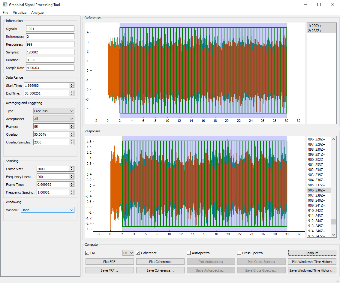
SignalProcessingGUI setup for the random excitation

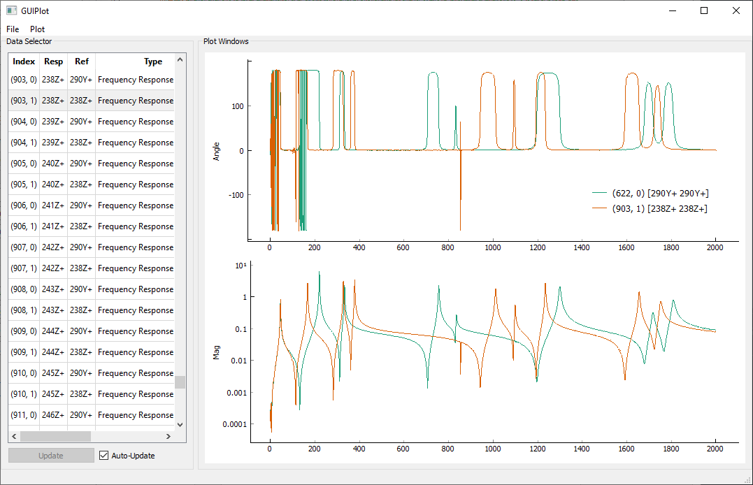
FRFs computed from the Random responses and excitation

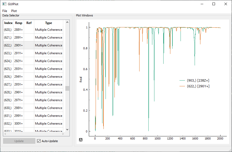
Multiple coherence computed from the Random responses and excitation

Note that now that we have two references, there are twice as many FRFs. In addition, the coherence being computed is now a Multiple Coherence function.

It can be illustrative to play around with some of the signal processing settings. For example, if we remove the Window by setting it back to Rectangle, the Multiple Coherence drops substantially. This is because coherence is a measure of how related the excitations and the responses are. With Random excitation, the responses are often due to forces that are outside the measurement frame, so from a signal processing standpoint, it seems like there are responses that are unrelated to the excitation, and the coherence therefore suffers. Applying the window lessens this effect, because it diminishes the forces and the responses at the edges of the frame, focusing instead on the forces and responses in the middle of the frame, which are more likely to be correlated to one another.

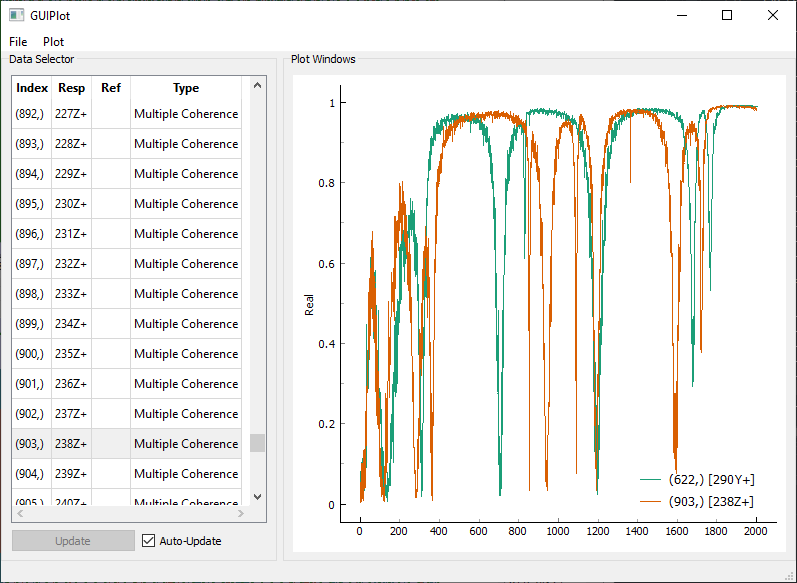
Multiple coherence computed from the Random responses and excitation with no window function.

We again pass the FRF data to the PolyPy curve fitter to fit modes. Because there are two references, there are now two columns of the FRF matrix and thus two singular values in the CMIF. Peaks in the CMIF still represent modes of the system, and multiple modes can be found at a given frequency if multiple curves of the CMIF peak at that frequency. This can be seen at the first mode of the system.

Due to the excitation from two directions, we now have excited more modes of the system. We therefore increase the Poly Order to 30 to 60 by 1. We keep the Data Type as Acceleration.

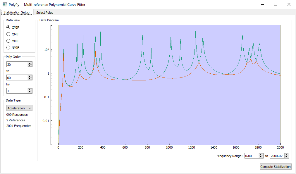
PolyPy setup for the Random excitation analysis showing two singular value curves on the CMIF.

We then look at the stability diagram. We must be sure to zoom into the areas where multiple peaks are shown in the CMIF to ensure that we select roots for both curves.

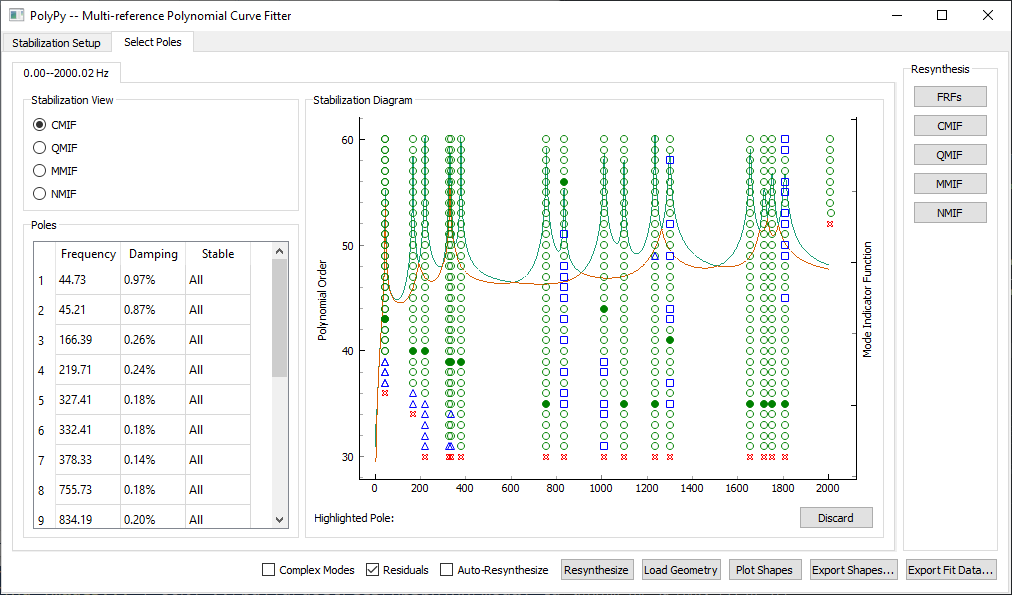
PolyPy stability for the Random excitation analysis. Note the closely spaced roots.

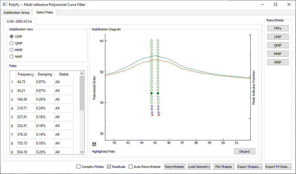
Zoom of the PolyPy stability for the Random excitation analysis at the first natural frequency. Note the two peaks with very similar roots.

We can then view the resynthesis to judge the adequacy of the fits. Note that both singular value curves should match if all repeated roots are captured.

CMIF resynthesis for the Random excitation analysis

We can then export the modes and exit the analysis. We will save the geometry for use in future analyses without needing to load the Exodus file again.

geometry.save('tuning_fork_geometry.npz')

Comparison of Excitation Techniques

We have now fit modes to each of the analyses. It would be beneficial to compare them not only against each other, but also against a linear eigensolution analysis from Sierra/SD.

We will first import our packages and then load in the Sierra/SD mode shapes.

import sdynpy as sdpy
import numpy as np

# Load in the Sierra/SD model and extract shapes
exodus_sd = sdpy.Exodus('tuning_fork_sd.e')
shapes_sd = sdpy.shape.from_exodus(exodus_sd)

We will then load in the geometry and shapes exported from our PolyPy analyses.

geometry = sdpy.Geometry.load('tuning_fork_geometry.npz')
shapes_sm_pr = sdpy.shape.load('tuning_fork_pseudorandom_shapes.npy')
shapes_sm_ra = sdpy.shape.load('tuning_fork_random_shapes.npy')

We will first compare shapes between the Random and Pseudorandom Excitations. We will compute a MAC matrix between the shapes to get correspondences, and then plot a mode table comparing the results.

# First compare the shapes from the solid mechanics runs
sm_mac = sdpy.shape.mac(shapes_sm_pr,shapes_sm_ra)
ax = sdpy.matrix_plot(sm_mac)
ax.set_ylabel('Pseudorandom Excitation')
ax.set_xlabel('MIMO Random Excitation')

# Print shape comparisons
pr_indices,ra_indices = np.where(sm_mac > 0.9)
print(sdpy.shape.shape_comparison_table(shapes_sm_pr[pr_indices], shapes_sm_ra[ra_indices]))

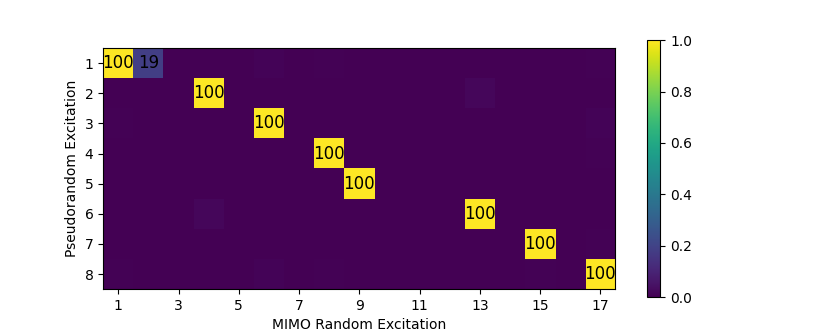
MAC between shapes extracted from Pseudorandom and Random analyses

|  Mode|  Freq 1 (Hz)|  Freq 2 (Hz)|  Freq Error|  Damp 1|  Damp 2|  Damp Error|  MAC|
|------|-------------|-------------|------------|--------|--------|------------|-----|
|     1|        44.66|        44.77|       -0.2%|   0.33%|   1.11%|      -70.4%|  100|
|     2|       219.70|       219.78|       -0.0%|   0.11%|   0.24%|      -52.4%|  100|
|     3|       332.43|       332.41|        0.0%|   0.11%|   0.17%|      -34.3%|  100|
|     4|       755.76|       755.71|        0.0%|   0.16%|   0.17%|       -6.8%|  100|
|     5|       834.21|       834.19|        0.0%|   0.18%|   0.19%|       -5.4%|  100|
|     6|      1299.19|      1299.19|        0.0%|   0.24%|   0.24%|       -0.6%|  100|
|     7|      1717.03|      1717.03|       -0.0%|   0.31%|   0.32%|       -3.0%|  100|
|     8|      1808.44|      1808.48|       -0.0%|   0.32%|   0.33%|       -2.4%|  100|

Note that the Random analysis was able to extract many more modes than the Pseudorandom due to the multiple simultaneous excitation forces that can be applied. Looking at modes that were extracted from both analyses, we see there was very good agreement in frequency between the two analyses. Significantly larger differences were found bewteen damping values particularly in the low frequency modes. This can be attributed to the Hann window, which artificially increases damping. The shape agreement was excellent.

We can also compare to results obtained from Sierra/SD. Note that the mesh used in this set of analyses was very coarse, with only two elements through the thickness. The Sierra/SD code uses by default fully-integrated hexahedral elements, whereas the Sierra/SM code uses by default under-integrated hexahedral elements, so the Sierra/SM results are expected to be softer in general than the Sierra/SD results. Were the meshes more refined, these differences would be lessened.

We will again plot the MAC matrix and get mode correspondences. We can also plot mode shapes for comparison.

# Now compare to SD analysis
sd_mac = sdpy.shape.mac(shapes_sd[shapes_sd.frequency < 2500],shapes_sm_ra)
ax = sdpy.matrix_plot(sd_mac)
ax.set_ylabel('SD Eigensolution')
ax.set_xlabel('SM MIMO Random Excitation')
sd_indices,ra_indices = np.where(sd_mac > 0.6)
print(sdpy.shape.shape_comparison_table(shapes_sd[sd_indices], shapes_sm_ra[ra_indices], damping_format=None))

geometry.plot_shape(shapes_sd[shapes_sd.frequency < 2500])
geometry.plot_shape(shapes_sm_ra)
geometry.plot_shape(shapes_sm_pr)

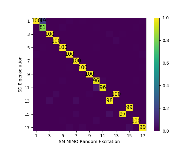
MAC between shapes extracted from Random and Eigensolution analyses

|  Mode|  Freq 1 (Hz)|  Freq 2 (Hz)|  Freq Error|  MAC|
|------|-------------|-------------|------------|-----|
|     1|        48.84|        44.77|        9.1%|  100|
|     2|        49.35|        45.23|        9.1%|   81|
|     3|       176.35|       166.38|        6.0%|  100|
|     4|       240.25|       219.78|        9.3%|  100|
|     5|       358.91|       327.32|        9.7%|  100|
|     6|       362.98|       332.41|        9.2%|  100|
|     7|       426.27|       378.33|       12.7%|  100|
|     8|       832.01|       755.71|       10.1%|  100|
|     9|       848.65|       834.19|        1.7%|  100|
|    10|      1129.70|      1011.06|       11.7%|   96|
|    11|      1383.31|      1098.41|       25.9%|   96|
|    12|      1445.70|      1299.19|       11.3%|  100|
|    13|      1457.41|      1234.26|       18.1%|   98|
|    14|      1860.25|      1717.03|        8.3%|   99|
|    15|      1937.92|      1655.41|       17.1%|   97|
|    16|      1947.79|      1751.61|       11.2%|  100|
|    17|      2015.65|      1808.48|       11.5%|   99|

Note that all modes in the bandwidth in the Sierra/SD model were also found in the Sierra/SM extractions, though with some frequency shifts. The one poor shape correlation occurs in the second mode, though this is more an artifact of the closely spaced modes in the random vibration test; the second mode ends up having some portion of the first mode, which is valid (for repeated eigenvalues, any linear combination of two eigenvectors is also an eigenvector).

Summary

This example problem showed how SDynPy can be used to interact with Sierra/SM results, treating the transient data as if it were test data and computing frequency response functions and fitting modes. In this way, nonlinear analysis data or other explicit analyses can be analyzed with structural dynamics techniques.

This example relied heavily on SDynPy’s graphical tools to compute frequency response functions and fit modes. Another option is to perform these same analyses via code, which allows more automation. If, for example, 5 different excitation strategies were analyzed instead of 2, it might have been worth scripting the FRF computation and mode fitting processes.