Substructuring with SDynPy
This document will demonstrate a topic that delves deeper into SDynPy’s capabilities, showcasing the workflow improvements and reduction of tediousness that can be gained by utilizing an integrated framework like SDynPy. This document will focus on performing dynamic substructuring with SDynPy, including the use of reduced-order models in the substructuring calculations. It will show how SDynPy can greatly simplify the bookkeeping operations that are prevalent in substructuring and reduced-order modeling operations. Unlike the previous documentation which used beam models with simple connection points, this document will utilize full 3D models to perform the substructuring calculations, which will require significantly more bookkeeping operations.
[1]:
import sdynpy as sdpy
import numpy as np
import matplotlib.pyplot as plt
Contents
Theory
Dynamic substructuring is the process of combining separate substructure models together to predict the dynamic response of the assembled structure [2]. In general, a dynamic system is represented by its Mass, Stiffness, and Damping Matrices (\(\mathbf{M}\), \(\mathbf{K}\), and \(\mathbf{C}\), respectively) in the typical second-order differential equation of motion.
Here \(\mathbf{u}\) are the physical response degrees of freedom and \(\mathbf{f}\) are the input force degrees of freedom. Each individual substructure can be represented by its own dynamic system. We can also represent multiple substructures as a block diagonal system of equations, with each block partition representing a different substructure.
In the case of previous equation, there is no connection between any of the substructures; they are effectively floating in space next to one another. To connect substructures to one another, we supplement this equation with constraint equations. These constraint equations are in general of the form \(\mathbf{B}\mathbf{u}=\mathbf{0}\). The \(\mathbf{B}\) matrix is often referred to as the Boolean matrix because it often contains only the values 0 and +/-1, though in general this is not strictly necessary. For example, if we wished to constrain the first degree of freedom in \(\mathbf{u}_1\) to the first degree of freedom in \(\mathbf{u}_2\) in this equation, the constraint equations would look like
which when expanded out would look like
The \(\mathbf{B}\) matrix will therefore have as many rows as constraints applied to the system and as many columns as degrees of freedom in the system.
To complicate matters, we are often not working with physical systems. We may be working with a reduced-order system in which the degrees of freedom in the system equations do not correspond one-to-one with a physical degree of freedom that should be coupled together. In this case, a reduction transformation between a reduced space and the physical space might be represented by the matrix \(\mathbf{R}\). For a modal system of equations, \(\mathbf{R}\) might be the mode shape matrix of the system. \(\mathbf{R}\) could also represent a Craig-Bampton or Guyan reduction transformation. The general equation of motion for such as system becomes
where \(\mathbf{\eta}\) are the generalized state degrees of freedom and \(\tilde{\mathbf{M}}\), \(\tilde{\mathbf{K}}\), and \(\tilde{\mathbf{C}}\) are the generalized mass, stiffness, and damping of the reduced system. In such a case where we wish to assemble many reduced substructures, our constraints must be applied to the generalized state degrees of freedom \(\tilde{\mathbf{B}}\mathbf{\eta}=\mathbf{0}\). In this case the Boolean matrix \(\tilde{\mathbf{B}}\) will generally not contain only 0 and +/-1. For example, to constrain the first two physical degrees of freedom of the first two systems as shown previously, the constraint equation matrix would be
where \({\mathbf{R}_1}^{(i)}\) represents the first row of the reduction transformation for the \(i\)th system.
It should be clear to the reader that the physical system shown in the reduced case is a special case of the equation shown in the physical case where the reduction transformation \(\mathbf{R}\) is simply the identity matrix \(\mathbf{I}\). Therefore, without loss of generality, this section will only consider the reduced system form from this point onward.
A final complication is the case where the analyst may not wish to constrain degrees of freedom directly (i.e. \({{u}_1}^{(1)} = {{u}_1}^{(2)}\)). Instead, the analyst may wish to apply constraints between many degrees of freedom. This is commonly done when there are not overlapping degrees of freedom between two substructures (e.g. the two substructures are finite element models created by two different groups without coincident nodes at the interface), or when performing experimental-to-analytical substructuring using the transmission simulator method [1]. In this case, rather than explicitly enforcing two degrees of freedom to move together, constraints are often applied to “shapes” of motion which are fit to the system in a least-squares sense.
In the general case of a reduced system, such a constraint equation for these shape-based constraints would look like
where \(\Phi^{(i)}\) represents the set of basis shapes used in the constraints partitioned to the degrees of freedom in the \(i\)th system and \(^+\) represents the pseudo-inverse of the matrix.
In the case where the reduction transformation for one of the systems is used as the constraint basis shapes (e.g. \({\Phi^{(2)}} = {\mathbf{R}}^{(2)}\)), which often happens when using the transmission simulator method, one may often see the constraint written as \begin{equation} \begin{bmatrix} {\mathbf{R}^{(2)}}^+ {\mathbf{R}}^{(1)} & -\mathbf{I} & \cdots & \mathbf{0} \end{bmatrix}\begin{bmatrix}{\mathbf{\eta}}^{(1)} \\ {\mathbf{\eta}}^{(2)} \\ \vdots \\ {\mathbf{\eta}}^{(n)}\end{bmatrix} = \mathbf{0} \end{equation}
Once the equations of motion and the constraint equations are set up, the analysis is not yet complete. One must construct a matrix \(\mathbf{L}\) that transforms the system of equations into a constrained set of generalized coordinates \(\mathbf{q}\) such that \(\mathbf{\eta} = \mathbf{L}\mathbf{q}\). These coordinates \(\mathbf{q}\) will be a reduced set of coordinates from the original coordinates \(\mathbf{\eta}\), which is intuitive due to the constraints applied to the system effectively removing degrees of freedom from the system. We can substitute this identity into the constraint equation
Noting that for the general case, the generalized coordinates \(\mathbf{q}\) can be nonzero; we therefore see that \(\tilde{\mathbf{B}}\mathbf{L} = \mathbf{0}\), or stated another way, \(\mathbf{L}\) must be the null space of \(\tilde{\mathbf{B}}\).
Once the matrix \(\mathbf{L}\) is found via the nullspace, the transformation can be applied to the equations of motion.
where
When a structural dynamic analysis is performed on this equation of motion, one must be aware that the output degrees of freedom are the generalized coordinates \(\mathbf{q}\). One can return to the reduced degrees of freedom by multiplying by \(\mathbf{L}\) and the physical degrees of freedom by multiplying by the respective reduction transformation \(\mathbf{R}\).
Using SDynPy for Substructuring
Almost immediately, we can imagine many ways implementing these equations could go wrong in practice. One must first assemble the systems into the block diagonal form, concatenating the systems together. One must keep track of the ordering of the degrees of freedom in each system, and then remember to apply the correct offset to the degree of freedom index when working with the concatenated system of equations (degree of freedom 1 in system (2) becomes degree of freedom 1 + \(m\) in the concatenated system, where \(m\) is the number of degrees of freedom in system (1)). One then must tediously assemble the \(\mathbf{B}\) matrix, identifying degrees of freedom that should be coupled together. If the 1s are not put into the correct columns of \(\mathbf{B}\), then the constraints will be applied incorrectly and the wrong degrees of freedom coupled together. Additionally, when viewed in matrix form, it is not immediately obvious if an error has been made.
Substructuring using reduced systems and softened constraints adds yet more bookkeeping steps to the calculations, creating another opportunity for errors could creep into the analysis. In this case, the \(\mathbf{B}\) matrix is no longer only 0 and +/-1, so it can be challenging to identify issues simply by inspecting the matrix. However, it is incredibly important that all degrees of freedom are kept track of throughout this process. When the result of a calculation is obtained, more bookkeeping and transformation steps are needed to transform from the reduced generalized coordinate space back to physical space. Overall, there is a huge potential for errors throughout these calculations, and with substructuring results being incredibly sensitive to small errors and changes in problem setup, it isn’t always clear if bad results are due to a poorly conceived problem or due to trivial bookkeeping errors along the way.
The substructuring capabilities in SDynPy are designed in a way to reduce as much as possible the chances for bookkeeping errors. Where bookkeeping error potential cannot be reduced due to manual operations involved (e.g. selecting which degrees of freedom to constrain), SDynPy gives users the capability to easily visualize their choices to more readily determine if they’ve made a mistake.
The most important object implemented by SDynPy for substructuring is the System object. The System object stores mass, stiffness, and damping matrices of a dynamic system, as well as the reduction transformation (\(\mathbf{M}\), \(\mathbf{K}\), \(\mathbf{C}\), and \(\mathbf{R}\), respectively; if no reduction transformation is needed, it is simply the identity matrix). Perhaps just as important, the System object also stores a list of physical degrees of freedom associated with the rows of the transformation matrix \(\mathbf{R}\), which also correspond to the rows and columns of the mass, stiffness, and damping matrices if the transformation is the identity matrix. Many bookkeeping operations in SDynPy are handled automatically because of these labeled degrees of freedom.
These degrees of freedom in a System object are stored as a CoordinateArray object in SDynPy. The CoordinateArray stores a node number and a direction (one of X+, X-, Y+, Y-, Z+, Z- or corresponding rotations) for each degree of freedom. In this way, SDynPy can keep track of which degree of freedom is which, as well as aid the user in bookkeeping operations (e.g. flipping the sign on the data if it was measured in the X- direction and the X+ direction is requested).
The degree of freedom information stored in the CoordinateArray is most meaningful when associated with a Geometry, which is the object SDynPy uses to store the spatial information associated with a test or an analysis. This spatial information is stored as positions of nodes in the geometry, as well as coordinate systems that define the orientations of sensors. Elements or lines can be added to the geometry to aid in visualization when it is plotted.
The ShapeArray object in SDynPy is traditionally used to represent mode shapes or deflection shapes, but it is also used to represent basis shapes that can be used in constraints \(\Phi\). ShapeArray objects similarly store their degree of freedom information as a CoordinateArray object, which allows for bookkeeping operations to be automated.
Exemplar Model
The example used in this paper is the Sierra/Structural Dynamics finite element model shown below. The model is built entirely from 8-node hexahedral elements, and its nodes can deform in three translational directions (no rotational degrees of freedom are present). The model is partitioned into three portions labeled A, B, and C.

Substructures used in this work consist of various portions of this model, shown in subsequent figures, with the end goal of reconstructing the dynamics of the full ABC system.
System A |
System A-2 |
System AC |
System C |
System BC |
|---|---|---|---|---|
|
|
|
|
|


System A-2 is equivalent geometrically to System A, but it has a finer mesh resolution.
The eigensolution of the finite element model is solved for the full System ABC case to provide truth frequencies and mode shapes against which the substructuring calculations can be compared. For each substructure, the mass and stiffness matrices are extracted from the finite element modeling software, so they can be used directly by SDynPy. The degree-of-freedom mapping is also exported from the finite element software, allowing a full System object to be constructed representing each substructure. These files can be downloaded here:
Mesh File:
Sierra Structural Dynamics Input Files:
Results Files:
System A Eigensolution Results
System A2 Eigensolution Results
System AC Eigensolution Results
System C Eigensolution Results
System BC Eigensolution Results
System ABC Eigensolution Results
To set up for the substructuring calculations, each model is read into the Python workspace. For each substructure, a System is created containing the substructure’s mass, stiffness, and degree-of-freedom information. A Geometry is also created for each substructure from its finite element mesh to facilitate plotting of results. Substructure System objects are stored in a Python dictionary called sys where the dictionary key was the system’s label in lower-case letters (e.g. sys['abc'] would provide the System object for System ABC). Similarly the Substructure Geometry objects are stored in a Python dictionary called geo where the dictionary key was again the system’s label in lower-case letters (e.g. geo['abc'] would provide the Geometry object for System ABC). This code assumes the files have been downloaded into a folder called assets in the current path. Users should update the file paths in the code snippet below if they have been downlaod into a different location.
[2]:
geo = {}
sys = {}
shp = {}
for label in ['abc','a','c','ac','bc','a2']:
exo = sdpy.Exodus(f"assets/block_{label}-eig.exo")
geo[label] = sdpy.geometry.from_exodus(exo)
geo[label].element.color = 1
shp[label] = sdpy.shape.from_exodus(exo)
sys[label] = sdpy.System.from_sierra_sd_mfile_output(
f"assets/block_{label}_Maa.m",f"assets/block_{label}_Kaa.m",
f"assets/block_{label}_gid.m",f"assets/block_{label}_ASetMap.m")
Substructuring Cases
The substructuring cases demonstrated in this paper are as follows:
Case 0: Constrain system A to ground to create a fixed-base model. This is not directly comparable to the truth system ABC, but it demonstrates how degrees of freedom can be fixed using SDynPy.
Case 1a: Constrain system A to system BC. This case will demonstrate a typical substructuring workflow using the
substructure_by_coordinatesubstructuring approach.Case 1b: Constrain system A to system BC. This case will demonstrate the
substructure_by_positionsubstructuring approach, which greatly simplifies the Case 1a workflow.Case 2: Constrain a modal representation of system A to a modal representation of system BC. This case will demonstrate substructuring using reduced-order models.
Case 3: Constrain a Craig-Bampton representation of system A to a Craig-Bampton representation of system BC. This case will demonstrate creating a Craig-Bampton model as well as the improved results compared to the modal modeling.
Case 4: Constrain a Craig-Bampton representation of system A to a modal representation of system BC. This case will demonstrate mixing different
Systemrepresentations.Case 5: Constrain system A-2 to system BC. This case will demonstrate constraining two components without common interface degrees of freedom, since A-2 has a different mesh resolution than system A.
Case 6: Constrain a modal representation of system AC to a modal representation of system BC and subtract off a modal representation of system C. This case will demonstrate shape-based constraints using
substructure_by_shapewhere system C exists in both substructures and must then be subtracted away.Case 7: Constrain an experimental modal representation of system AC to an analytical modal representation of system BC and subtract off an analytical modal representation of system C. This case will demonstrate a typical experimental/analytical transmission simulator method substructuring case where the experimental substructure has a limited bandwidth and measurement point resolution.
Case 0: Constrained to Ground
Case 0 will demonstrate fixing of substructure A to ground. While it is not directly comparable to the truth system ABC, fixing degrees of freedom is a common operation in substructuring calculations, and therefore it was desirable to demonstrate in this paper.
The first step in this process is to determine the degrees of freedom that should be fixed. In the case of System A, the end we wish to fix happens to lie with its X-coordinate at a value of 0.0625. Therefore, we can use this quantity and the geometry operations available in SDynPy to select for first the nodes that lie at this X-coordinate, and then select the degrees of freedom assocated with these nodes.
As mentioned previously, certain aspects of substructuring are necessarily manual; selection of degrees of freedom to use in constraints is often one of those aspects. Therefore, it is important to be able to quickly visualize the results of the operation to ensure that the correct result is obtained. In SDynPy, CoordinateArray objects can be easily plotted on Geometry objects using the plot_coordinate method.
[3]:
fixed_end_nodes = geo['a'].node.id[
abs(geo['a'].global_node_coordinate()[:,0] - 0.0625) < 0.01
]
fixed_dofs = sdpy.coordinate_array(fixed_end_nodes,['X+','Y+','Z+'],force_broadcast=True)
geo['a'].plot_coordinate(fixed_dofs,arrow_scale=0.025,label_dofs=True,opacity=0.25)
[3]:
<sdynpy.core.sdynpy_geometry.GeometryPlotter at 0x1f60ca60950>

When substructuring directly using degrees of freedom, we will generally utilize the substructure_by_coordinate method in SDynPy. This method requires us to provide pairs of degrees of freedom to constrain together. If, instead of constraining two degrees of freedom together, we instead wish to constrain one degree of freedom to ground, we pair that degree of freedom with None instead of a second degree of freedom.
[4]:
constraint_list = [(dof,None) for dof in fixed_dofs]
At this point, performing the substructuring is as simple as calling the substructure_by_coordinate method on the System object to apply the constraints.
[5]:
constrained_system = sys['a'].substructure_by_coordinate(constraint_list)
In less than 10 lines of code, we have performed a substructuring calculation in SDynPy with our existing System object, and over half of those lines were selecting the constraint degrees of freedom.
Throughout this paper, the author would encourage the reader to think about all of the operations SDynPy is performing in the background that have potential for bookkeeping errors. In the first code snippet, we search for nodes in our geometry with a specific X-coordinate. We then map that to a node ID number. We then search through the System object, searching for the rows and columns of the matrices corresponding to the X, Y, and Z degrees of freedom associated with each of those nodes, and set up the constraint matrix appropriately for those degrees of freedom. We then compute the constraint matrix and apply the constraints to the system, producing reduced system matrices.
However, the responsible reader should then question: “How do I know SDynPy is doing all of these operations correctly in the background?” As with manual operations such as selecting degrees of freedom, whenever SDynPy is performing a good deal of work behind the scenes, the author’s best practice is to somehow visualize the results to ensure that they make sense. Once again, SDynPy provides visualization tools that make it almost trivial to verify that the operations were performed successfully. In this case, we will simply compute the eigensolution of our system and plot the mode shapes using plot_shape. If we see that the mode shapes look fixed at the base, we can be reasonably sure that the computations were performed correctly.
[6]:
num_modes = 50
constrained_shapes = constrained_system.eigensolution(num_modes)
geo['a'].plot_shape(constrained_shapes)
[6]:
<sdynpy.core.sdynpy_geometry.ShapePlotter at 0x1f60ca628d0>

While performing this operation, the author would again encourage the reader to think about their typical substructuring workflows and imagine what it would take to compute the eigensolution of this reduced system and plot the mode shapes. One must first compute the eigensolution of the reduced matrices. Then one must transform the mode shapes from the reduced space back to the physical space. Finally, one must map each of those mode shape coefficients to a displacement vector in 3D space and displace the corresponding nodes of the model by that amount in the correct direction. Depending on the plotting software used, these shapes may not be interactive nor animated. In SDynPy, the eigensolution can be computed in one line of code using the eigensolution method, and the mode shapes plotted in an animated, interactive environment with a second line of code using the plot_shape method.
SDynPy’s System object tracks the reduction transformation applied to each system and will therefore transform result of calculations such as eigensolution back to physical degrees of freedom, which can then be plotted. From this shape, one can verify that the end of the structure has been fixed.
Case 1a: Constrain System A to System BC
Case 1 will demonstrate perhaps the most common substructuring calculation; we have two substructures, A and BC, which have common interface degrees of freedom. Each constraint we will apply will constrain one degree of freedom from system A to move identically to the corresponding degree of freedom in System B. This case will be presented to show the full substructuring workflow, and the subsequent case will show how we can significantly streamline the analysis.
To start, we have sys['a'] and sys['bc'] as separate System objects. The first step, then, is to concatenate the systems together to the block diagonal form. However, we must be careful; each of sys['a'] and sys['bc'] are tracking the degrees of freedom associated with their matrices, and depending on the sources of the System objects, these may have conflicting degree of freedom labels (each System, for example, may have a node 1, and therefore may have a degree of freedom 1X+). Therefore, when we concatenate systems together, it is best practice to provide an “offset value” to ensure no node conflicts.
While we could of course examine the System objects directly to identify the maximum degree of freedom in the system, this would be a relatively manual procedure which SDynPy aims to avoid. Instead, we will use the overlay_geometries method, which in addition to identifying an offset value that ensures no conflicts between geometry, also provides us with a Geometry which, at the end of our analysis, we can use to plot our results. We ensure that we specify the return_node_id_offset=True keyword argument so the overlay_geometries method returns the offset value. Here we also specify the color_override keyword argument to color the two substructures differently. As always, we should plot to ensure things make sense.
[7]:
combined_geometry,node_offset = sdpy.Geometry.overlay_geometries(
[geo['a'],geo['bc']],return_node_id_offset=True,color_override=[1,7])
combined_geometry.plot();

Now when we concatenate our systems together, we can pass this node_offset value as an optional argument, and the concatenate method will automatically assign the identical offset to our systems as the geometry; this keeps the degrees of freedom in the concatenated System object consistent with the combined Geometry object which will facilitate the visualization of the eventual results.
[8]:
combined_system = sdpy.System.concatenate([sys['a'],sys['bc']],coordinate_node_offset=node_offset)
One thing to note, however, is that the two substructures within the concatenated System object are not connected to one another in any way. For example, we can compute an eigensolution and plot_shape to visualize the mode shapes, which appear to be completely independent from one another. The motion between the two substructures is discontinuous, proving there is no constraint between the two as of yet.
[9]:
combined_shapes = combined_system.eigensolution(num_modes)
combined_geometry.plot_shape(combined_shapes)
[9]:
<sdynpy.core.sdynpy_geometry.ShapePlotter at 0x1f60cb476e0>

This case will again use the substructure_by_coordinate method, meaning we need to construct pairs of degrees of freedom that we will constrain together. Getting the interface nodes from System A we have already shown in Case 0:
[10]:
constraint_nodes = geo['a'].node.id[
abs(geo['a'].global_node_coordinate()[:,0] - 0.0625) < 0.01
]
constraint_dofs = sdpy.coordinate_array(constraint_nodes,['X+','Y+','Z+'],force_broadcast=True)
geo['a'].plot_coordinate(constraint_dofs,arrow_scale=0.025,label_dofs=True,opacity=0.25)
[10]:
<sdynpy.core.sdynpy_geometry.GeometryPlotter at 0x1f60cb45910>
To find the corresponding degrees of freedom from System BC, we can use the map_coordinate method. This method searches a second geometry for the degrees of freedom most closely aligned from a first geometry. With the keyword argument node_map='position', it will automatically find the closest node in the second geometry to the first geometry, and then find the degree of freedom at that node that is pointing in the same direction as the provided degree of freedom. If for example, a substructure were defined in a different local coordinate system (e.g., X+ to Y+) or different polarity (e.g., X+ to X-), the map_coordinate method would handle those coordinate system transformations to identify the correct degree of freedom pairing. Here is another instance where it is a good idea to verify that the mapping has been performed correctly.
[11]:
corresponding_dofs = geo['a'].map_coordinate(constraint_dofs, geo['bc'], node_map='position')
# We can verify that they are correct correspondences, plot one of them as a spot check
correspondence_index = 10
geo['a'].plot_coordinate(constraint_dofs[correspondence_index],opacity=0.25)
geo['bc'].plot_coordinate(corresponding_dofs[correspondence_index],opacity=0.25)
[11]:
<sdynpy.core.sdynpy_geometry.GeometryPlotter at 0x1f618139d00>

We can then construct the entire constraint list containing pairs of degrees of freedom. Using NumPy indexing operations such as newaxis and methods such as concatenate can help us quickly construct this array. We must also recognize that we have performed these degree of freedom operations on the original Geometry objects, not the concatenated Geometry. Therefore, we must remember to apply our node_offset to the node numbers.
[12]:
constraint_list = np.concatenate((constraint_dofs[:,np.newaxis],
corresponding_dofs[:,np.newaxis]),axis=-1)
constraint_list.node = constraint_list.node + [node_offset,2*node_offset]
At this point, we can then apply the constraints to the concatenated System object in the same way we did previously with the substructure_by_coordinate method.
[13]:
constrained_system = combined_system.substructure_by_coordinate(constraint_list)
constrained_shapes = constrained_system.eigensolution(num_modes)
Of course, we should check our work by plotting some mode shapes and comparing to the truth model from the finite element model. SDynPy has many features for comparing different sets of data. One might plot a modal assurance criteria matrix, overlay mode shapes, or plot frequencies in a table. These are done here, but for brevity they will not be discussed in depth, as this document is meant to focus on the substructuring operations. We will write a generic function to perform these operations, so it can be called for each case examined in this document.
[14]:
def compare_to_truth(case_name,truth_geo,truth_shapes,compare_geo,compare_shapes):
num_shapes = np.min([truth_shapes.size,compare_shapes.size])
# Set up comparisons to the truth model
check_nodes = compare_geo.node_by_global_position(truth_geo.global_node_coordinate())
truth_node_ids = truth_geo.node.id
# Make sure that a single check node is not associated with more than one
# truth node
if check_nodes.id.size != np.unique(check_nodes.id).size:
# Go through and find the closest geometry node to each check node
check_node_ids = np.unique(check_nodes.id)
check_node_truth_pair = truth_geo.node_by_global_position(compare_geo.global_node_coordinate(check_node_ids))
check_nodes = compare_geo.node_by_global_position(truth_geo.global_node_coordinate(check_node_truth_pair.id))
truth_node_ids = check_node_truth_pair.id
truth_map = sdpy.id_map(
check_nodes.id,
truth_node_ids
)
compare_shapes = compare_shapes.copy()
print('{:} Results:'.format(case_name))
# Find corresponding mode shapes
full_mac = sdpy.shape.mac(truth_shapes[6:num_shapes].reduce(truth_node_ids),
compare_shapes[6:num_shapes].reduce(truth_map.from_ids),truth_map)
truth_corr,compare_corr = np.where(full_mac > 0.4)
print(sdpy.shape.shape_comparison_table(
compare_shapes[compare_corr+6].reduce(truth_map.from_ids),
truth_shapes[truth_corr+6].reduce(truth_node_ids),
damping_format = None, node_id_map=truth_map.inverse()))
alignment = sdpy.shape.shape_alignment(
truth_shapes[truth_corr+6].reduce(truth_node_ids),
compare_shapes[compare_corr+6].reduce(truth_map.from_ids),truth_map)
compare_shapes.shape_matrix[compare_corr+6] = compare_shapes.shape_matrix[compare_corr+6]*alignment[:,np.newaxis]
combined_geometry,combined_shapes = sdpy.shape.overlay_shapes(
[truth_geo,compare_geo],
[truth_shapes[truth_corr+6],compare_shapes[compare_corr+6]],
[1,7])
combined_shapes.comment1 = case_name
combined_shapes.comment2 = 'Truth: Blue, Substructured: Green'
for shape1,shape2,c in zip(
truth_shapes[truth_corr+6].reduce(truth_node_ids),
compare_shapes[compare_corr+6].reduce(truth_map.from_ids),
combined_shapes):
freq_error = (shape2.frequency-shape1.frequency)/shape1.frequency*100
mac = sdpy.shape.mac(shape1[np.newaxis],shape2[np.newaxis],truth_map)[0,0]*100
error_string = f'Truth: {shape1.frequency:0.2f} Hz; Substructured: {shape2.frequency:0.2f} Hz'
c.comment3 = error_string
error_string = f'Error: {freq_error:0.1f}%; MAC: {mac:0.2f}'
c.comment4 = error_string
plotter = combined_geometry.plot_shape(combined_shapes,undeformed_opacity=0,deformed_opacity=0.25)
ax = sdpy.correlation.matrix_plot(full_mac,text_size=4)
ax.set_title(case_name)
return plotter, ax, sdpy.shape.shape_comparison_table(
compare_shapes[compare_corr+6].reduce(truth_map.from_ids),
truth_shapes[truth_corr+6].reduce(truth_node_ids),
damping_format = None, node_id_map=truth_map.inverse(),table_format='markdown')
We can call this function with our results to generate the visualizations.
[15]:
comparison_plotter, mac_ax, frequency_table = compare_to_truth(
'Case 1a', geo['abc'], shp['abc'],
combined_geometry, constrained_shapes)
Case 1a Results:
Mode Freq 1 (Hz) Freq 2 (Hz) Freq Error MAC
1 463.46 463.46 -0.0% 100
2 585.95 585.95 0.0% 100
3 750.96 750.96 0.0% 100
4 834.17 834.17 0.0% 100
5 1368.49 1368.49 0.0% 100
6 1434.50 1434.50 0.0% 100
7 1458.50 1458.50 0.0% 100
8 1665.14 1665.14 0.0% 100
9 1727.17 1727.17 0.0% 100
10 2021.03 2021.03 0.0% 100
11 2766.90 2766.90 0.0% 100
12 3138.37 3138.37 0.0% 100
13 3432.29 3432.29 0.0% 100
14 3765.91 3765.91 0.0% 100
15 3870.86 3870.86 0.0% 100
16 4062.56 4062.56 -0.0% 100
17 4250.85 4250.85 0.0% 100
18 4312.22 4312.22 0.0% 100
19 4319.28 4319.28 0.0% 100
20 4947.56 4947.56 0.0% 100
21 5193.05 5193.05 0.0% 100
22 5687.49 5687.49 0.0% 100
23 6198.35 6198.35 0.0% 100
24 6210.73 6210.73 0.0% 100
25 6945.25 6945.25 0.0% 100
26 7102.79 7102.79 0.0% 100
27 7246.99 7246.99 0.0% 100
28 7397.53 7397.53 0.0% 100
29 7729.57 7729.57 0.0% 100
30 7992.09 7992.09 0.0% 100
31 8049.50 8049.50 0.0% 100
32 8310.52 8310.52 0.0% 100
33 8860.38 8860.38 0.0% 100
34 9069.66 9069.66 0.0% 100
35 9263.32 9263.32 0.0% 100
36 9591.93 9591.93 0.0% 100
37 9875.70 9875.70 0.0% 100
38 10060.16 10060.16 0.0% 100
39 10307.29 10307.29 0.0% 100
40 10369.17 10369.17 0.0% 100
41 10758.10 10758.10 0.0% 100
42 11618.55 11618.55 0.0% 100
43 11800.98 11800.98 0.0% 100
44 12079.93 12079.93 0.0% 100


The substructured model is identical to the truth model, suggesting that all substructuring constraints and transformations back to physical space were applied correctly by SDynPy.
Case 1b: Constrain System A to System BC
In the previous subsection, we saw the typical substructuring workflow: concatenate the System objects together, select degrees of freedom by closest position, apply constraints, and visualize results. However, because this type of substructuring calculation, where degrees of freedom already exist co-located spatially in the two systems, is common, SDynPy has a shortcut method: substructure_by_position. This method automatically searches out common degrees of freedom in the System objects and applies constraints between them, meaning the entirety of Case 1a can be performed in a single function call.
[16]:
# Perform the substructuring
constrained_system, combined_geometry = sdpy.System.substructure_by_position(
[sys['a'],sys['bc']],
[geo['a'],geo['bc']])
# Compare results
constrained_shapes = constrained_system.eigensolution(num_modes)
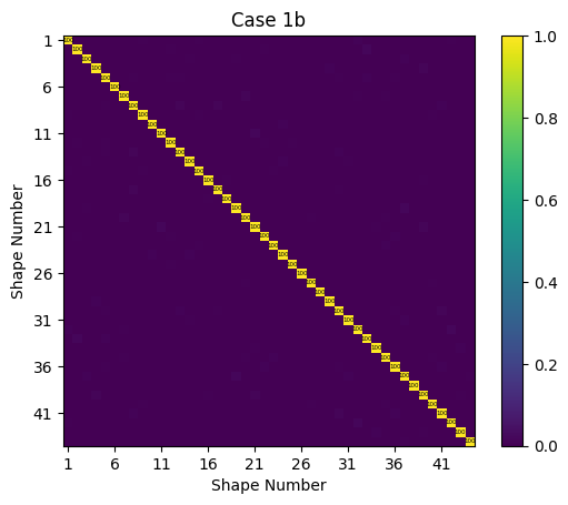
comparison_plotter, mac_ax, latex_table = compare_to_truth(
'Case 1b', geo['abc'], shp['abc'],
combined_geometry, constrained_shapes)
Case 1b Results:
Mode Freq 1 (Hz) Freq 2 (Hz) Freq Error MAC
1 463.46 463.46 -0.0% 100
2 585.95 585.95 -0.0% 100
3 750.96 750.96 -0.0% 100
4 834.17 834.17 -0.0% 100
5 1368.49 1368.49 0.0% 100
6 1434.50 1434.50 0.0% 100
7 1458.50 1458.50 0.0% 100
8 1665.14 1665.14 0.0% 100
9 1727.17 1727.17 0.0% 100
10 2021.03 2021.03 0.0% 100
11 2766.90 2766.90 0.0% 100
12 3138.37 3138.37 0.0% 100
13 3432.29 3432.29 0.0% 100
14 3765.91 3765.91 0.0% 100
15 3870.86 3870.86 0.0% 100
16 4062.56 4062.56 0.0% 100
17 4250.85 4250.85 0.0% 100
18 4312.22 4312.22 0.0% 100
19 4319.28 4319.28 0.0% 100
20 4947.56 4947.56 0.0% 100
21 5193.05 5193.05 0.0% 100
22 5687.49 5687.49 0.0% 100
23 6198.35 6198.35 0.0% 100
24 6210.73 6210.73 0.0% 100
25 6945.25 6945.25 0.0% 100
26 7102.79 7102.79 0.0% 100
27 7246.99 7246.99 0.0% 100
28 7397.53 7397.53 0.0% 100
29 7729.57 7729.57 0.0% 100
30 7992.09 7992.09 0.0% 100
31 8049.50 8049.50 0.0% 100
32 8310.52 8310.52 0.0% 100
33 8860.38 8860.38 0.0% 100
34 9069.66 9069.66 0.0% 100
35 9263.32 9263.32 0.0% 100
36 9591.93 9591.93 0.0% 100
37 9875.70 9875.70 0.0% 100
38 10060.16 10060.16 0.0% 100
39 10307.29 10307.29 0.0% 100
40 10369.17 10369.17 0.0% 100
41 10758.10 10758.10 0.0% 100
42 11618.55 11618.55 0.0% 100
43 11800.98 11800.98 0.0% 100
44 12079.93 12079.93 0.0% 100

Case 2: Constrain a Modal Representation of System A to a Modal Representation of System BC
The previous cases showed substructuring calculations consisting of “full” or “physical” System objects: each row and column of the mass and stiffness matrices represents a physical degree of freedom in the system. However, very often when we perform substructuring calculations, the goal is to combine reduced-order models of the substructures in order to reduce the size of the final assembled model. This case will demonstrate substructuring with modal models of the two systems. Note this case is expected to perform poorly due to free modes of the system not providing an adequate basis set of shapes for substructuring calculations.
To begin, we will construct modal systems for Systems A and BC. We have seen that we can compute modes with the eigensolution method. Once we have modes of the system, we can then compute a modal system by using the system method. In this case, we use 105 modes of each substructure to construct the reduced systems.
[17]:
modal_sys_a = sys['a'].eigensolution(105).system()
modal_sys_bc = sys['bc'].eigensolution(105).system()
We can visualize the structure of a System object using its spy method, which plots the connectivity of the system matrices as well as the transformations. We can, for example, compare the full system against the reduced system.
[18]:
sys['a'].spy();
modal_sys_a.spy();
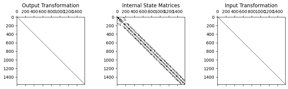
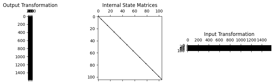
The top figure shows the physical system matrices; note the diagonal transformation matrices, which are the identity matrix, and the non-diagonal state matrices, which shows coupling between the various physical degrees of freedom. The bottom figure shows the modal system matrices; note the full transformation matrices, which are the mode shape matrices, and the diagonal state matrices, which is expected from a modal solution. Note also that the physical system shows over 1500 degrees of freedom, while the modal system only shows 105 degrees of freedom, which is the number of modes used to construct the system.
With SDynPy handling all of the transformation effects, we could of course compute the modes of the reduced systems using eigensolution and plot them using plot_shape, and we would expect to see the identical modes used to compute the modal system. This also means we can simply pass these reduced systems to the same substructuring algorithms, and the transformations will be handled automatically for us. For example, we can simply pass the modal representations modal_sys_a and modal_sys_bc to the substructure_by_position method, and we are done.
[19]:
# Perform substructuring
constrained_system, combined_geometry = sdpy.System.substructure_by_position(
[modal_sys_a,modal_sys_bc],
[geo['a'],geo['bc']])
# Compare results
constrained_shapes = constrained_system.eigensolution(num_modes)
comparison_plotter, mac_ax, latex_table = compare_to_truth('Case 2', geo['abc'], shp['abc'],
combined_geometry, constrained_shapes)
Case 2 Results:
Mode Freq 1 (Hz) Freq 2 (Hz) Freq Error MAC
1 712.21 463.46 53.7% 52
2 721.52 463.46 55.7% 41
3 712.21 585.95 21.5% 44
4 721.52 585.95 23.1% 55
5 977.59 750.96 30.2% 95
6 1134.62 834.17 36.0% 98
7 1710.81 1368.49 25.0% 55
8 1727.99 1434.50 20.5% 97
9 1662.56 1458.50 14.0% 95
10 2729.07 1727.17 58.0% 71
11 2947.27 2021.03 45.8% 85
12 2986.11 2766.90 7.9% 96
13 3434.21 3138.37 9.4% 96
14 2829.45 3432.29 -17.6% 58
15 4125.19 3765.91 9.5% 91
16 4800.14 4062.56 18.2% 60
17 4746.24 4250.85 11.7% 85
18 5128.22 4312.22 18.9% 60
19 5934.53 4319.28 37.4% 43
20 5748.11 4947.56 16.2% 59
21 7030.11 5193.05 35.4% 73
22 6289.84 5687.49 10.6% 77
23 7049.18 6198.35 13.7% 56
24 7720.80 6210.73 24.3% 53
25 8627.38 7102.79 21.5% 47
26 9629.19 8049.50 19.6% 49
27 8851.74 8860.38 -0.1% 53
28 8965.10 9069.66 -1.2% 40
29 10330.90 9069.66 13.9% 41
30 10246.00 9263.32 10.6% 47
31 10015.11 9591.93 4.4% 46
32 11803.94 9875.70 19.5% 44
33 8627.38 10060.16 -14.2% 41
34 11761.74 10369.17 13.4% 58
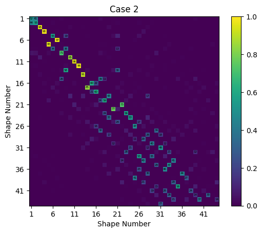

Similar to the previous case, the substructure_by_position method will use the geometry to automatically pair degrees of freedom for constraining. It will then compute and apply the constraints to the System. We see in this case that it also automatically handles the reduction transformation as part of this calculation. However, in this case, the modal representation of these systems does not provide a good basis set for substructuring. For example, in System A there is no strain at the interface in any free mode of the structure. Therefore, when we substructure using these shapes, there is also no strain in any shape at the interface of the assembled system, even though the assembled system should have strain in the interface. The result is a poor match to the true assembled system. The MAC matrix shows very few strong correspondences; the overlaid mode shapes shows significant divergences, and the natural frequencies show up to 50% error at mode shapes that look similar.
Case 3: Constrain a Craig-Bampton representation of system A to a Craig-Bampton representation of system BC
We saw in the previous case that poor results were obtained when using a reduced-order model consisting of the free modes of the substructures. However, other reduction bases can provide better results. For example, the well-known Craig-Bampton representation is a very good reduced-order model for substructuring applications.
To construct a Craig-Bampton representation in SDynPy, one must specify the degrees of freedom to use as the interface degrees of freedom, from which static deflection shapes will be constructed, as well as the number of fixed-base modes to keep. We will start by selecting the interface degrees of freedom, which follows a similar procedure to the one used to select the degrees of freedom to constrain in Case 1a.
[20]:
constraint_nodes = geo['a'].node.id[
abs(geo['a'].global_node_coordinate()[:,0] - 0.0625) < 0.01
]
constraint_dofs = sdpy.coordinate_array(constraint_nodes,['X+','Y+','Z+'],force_broadcast=True)
corresponding_dofs = geo['a'].map_coordinate(constraint_dofs, geo['bc'], node_map='position')
We can then construct the Craig-Bampton substructures using the reduce_craig_bampton method.
[21]:
num_cbr_modes = 30
sys_cb_a = sys['a'].reduce_craig_bampton(constraint_dofs, num_cbr_modes)
sys_cb_bc = sys['bc'].reduce_craig_bampton(corresponding_dofs, num_cbr_modes)
To ensure that SDynPy has properly constructed the transformation, we can extract the transformation shapes with the transformation_shapes method and plot them with the plot_shape method. The fixed-base shapes should show no motion at the interface degrees of freedom, and each of the static deflection shapes should show unit deflection of only one interface degree of freedom.
[22]:
geo['a'].plot_shape(sys_cb_a.transformation_shapes())
geo['bc'].plot_shape(sys_cb_bc.transformation_shapes())
[22]:
<sdynpy.core.sdynpy_geometry.ShapePlotter at 0x1f7644b7c80>


We can then constrain the reduced substructures as before.
[23]:
# Perform the constraints
constrained_system, combined_geometry = sdpy.System.substructure_by_position(
[sys_cb_a,sys_cb_bc],
[geo['a'],geo['bc']])
constrained_shapes = constrained_system.eigensolution(num_modes)
comparison_plotter, mac_ax, latex_table = compare_to_truth('Case 3', geo['abc'], shp['abc'],
combined_geometry, constrained_shapes)
Case 3 Results:
Mode Freq 1 (Hz) Freq 2 (Hz) Freq Error MAC
1 463.46 463.46 0.0% 100
2 585.96 585.95 0.0% 100
3 750.96 750.96 0.0% 100
4 834.17 834.17 0.0% 100
5 1368.52 1368.49 0.0% 100
6 1434.50 1434.50 0.0% 100
7 1458.52 1458.50 0.0% 100
8 1665.30 1665.14 0.0% 100
9 1727.18 1727.17 0.0% 100
10 2021.07 2021.03 0.0% 100
11 2767.00 2766.90 0.0% 100
12 3140.80 3138.37 0.1% 100
13 3432.48 3432.29 0.0% 100
14 3767.55 3765.91 0.0% 100
15 3871.50 3870.86 0.0% 100
16 4063.53 4062.56 0.0% 100
17 4251.80 4250.85 0.0% 100
18 4312.29 4312.22 0.0% 100
19 4319.99 4319.28 0.0% 100
20 4948.01 4947.56 0.0% 100
21 5195.45 5193.05 0.0% 100
22 5713.39 5687.49 0.5% 100
23 6213.95 6198.35 0.3% 100
24 6215.22 6210.73 0.1% 100
25 6945.63 6945.25 0.0% 100
26 7110.41 7102.79 0.1% 100
27 7247.83 7246.99 0.0% 100
28 7398.35 7397.53 0.0% 100
29 7732.32 7729.57 0.0% 100
30 8101.14 7992.09 1.4% 97
31 8052.87 8049.50 0.0% 100
32 8336.37 8310.52 0.3% 99
33 8877.18 8860.38 0.2% 99
34 9108.49 9069.66 0.4% 99
35 9324.33 9263.32 0.7% 99
36 9627.06 9591.93 0.4% 98
37 9914.18 9875.70 0.4% 99
38 10095.29 10060.16 0.3% 98
39 10308.96 10307.29 0.0% 100
40 10392.18 10369.17 0.2% 99
41 11756.93 10758.10 9.3% 62
42 12108.51 12079.93 0.2% 99
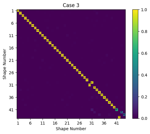

We see the results using Craig-Bampton substructure models are much better than the results obtained using free modes of the substructures, noting that Case 2 and Case 3 both used substructure systems with the same number of degrees of freedom. The substructures in Case 2 used 105 free modes of the structures, and the substructures in Case 3 used substructures with 75 interface degrees of freedom (25 nodes each with three translational degrees of freedom) and 30 fixed-interface modes.
Case 4: Constrain a Craig-Bampton Representation of System A to a Modal Representation of System BC
It should be noted that there is no requirement that both systems be physical systems, both systems be modal systems, or both systems be Craig-Bampton systems. For example, we can easily constrain our modal substructure BC with our Craig-Bampton substructure A. Whatever transformation matrix the System object has will be used in the substructuring procedure.
[24]:
# Perform the constraints
constrained_system, combined_geometry = sdpy.System.substructure_by_position(
[sys_cb_a,modal_sys_bc],
[geo['a'],geo['bc']])
constrained_shapes = constrained_system.eigensolution(num_modes)
comparison_plotter, mac_ax, latex_table = compare_to_truth('Case 4', geo['abc'], shp['abc'],
combined_geometry, constrained_shapes)
Case 4 Results:
Mode Freq 1 (Hz) Freq 2 (Hz) Freq Error MAC
1 483.69 463.46 4.4% 100
2 605.51 585.95 3.3% 100
3 758.37 750.96 1.0% 100
4 842.58 834.17 1.0% 100
5 1378.94 1368.49 0.8% 100
6 1461.73 1434.50 1.9% 100
7 1459.36 1458.50 0.1% 100
8 1677.23 1665.14 0.7% 100
9 1780.78 1727.17 3.1% 100
10 2071.32 2021.03 2.5% 100
11 2769.30 2766.90 0.1% 100
12 3172.44 3138.37 1.1% 100
13 3440.45 3432.29 0.2% 100
14 3801.95 3765.91 1.0% 100
15 3927.86 3870.86 1.5% 100
16 4113.57 4062.56 1.3% 98
17 4292.42 4250.85 1.0% 100
18 4351.40 4312.22 0.9% 98
19 4346.18 4319.28 0.6% 100
20 4976.46 4947.56 0.6% 100
21 5207.21 5193.05 0.3% 100
22 5785.22 5687.49 1.7% 99
23 6261.80 6198.35 1.0% 100
24 6233.36 6210.73 0.4% 100
25 7009.95 6945.25 0.9% 100
26 7240.32 7102.79 1.9% 99
27 7325.50 7246.99 1.1% 99
28 7476.34 7397.53 1.1% 98
29 7774.79 7729.57 0.6% 100
30 8108.13 7992.09 1.5% 99
31 8193.71 8049.50 1.8% 98
32 8374.59 8310.52 0.8% 100
33 8878.71 8860.38 0.2% 100
34 9111.74 9069.66 0.5% 100
35 9377.93 9263.32 1.2% 99
36 9659.11 9591.93 0.7% 100
37 9932.52 9875.70 0.6% 100
38 10201.21 10060.16 1.4% 94
39 10339.42 10307.29 0.3% 93
40 10439.10 10369.17 0.7% 99
41 10894.67 10758.10 1.3% 99
42 11707.66 11618.55 0.8% 99
43 11890.10 11800.98 0.8% 99
44 12430.86 12079.93 2.9% 98
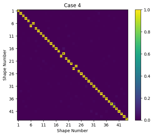

Interestingly, this results in significantly improved results over Case 2, even through a substructure with free modes are used. This is likely due to there being strain at the interface in the free mode shapes of System BC, unlike the interface in the free modes of System A.
Case 5: Constrain System A-2 to System BC
All previous cases have considered the situation where the degrees of freedom to be combined between the substructures are directly co-located. However, there are cases when the degrees of freedom that must be constrained do not map one-to-one across the substructuring interface. This can occur when different groups build the substructure models, or when experimental models are used.
In this case, we will consider the problem where we again constrain System A to System BC. However, in this case, we use System A-2, which is geometrically the same as System A, except it has a finer mesh resolution, so the degrees of freedom do not map one-to-one. Utilizing the substructure_by_position method would result in poor results, because only the nodes at the corners of System A-2 would be constrained to System BC.
[25]:
combined_geometry,node_offset = sdpy.Geometry.overlay_geometries(
[geo['a2'],geo['bc']],return_node_id_offset=True,color_override=[1,7])
combined_geometry.plot(show_edges=True);

In this case, we will use a set of shapes to provide the constraints. We effectively fit motions at the interface to a set of basis shapes, and then constrain those shape coefficients to one another.
Often when using shape-based constraints, a physically-based set of shapes is used, for example, the mode shapes of one of the structures. However, we have seen in Case 2 that the free shapes do not provide a good basis set of shapes for the motions seen at the interface. Therefore, we will instead use Legendre Polynomials as the basis functions. These polynomials look somewhat like plate bending modes, and therefore should adequately capture the motions of the interfaces. The SciPy package
contains Legendre polynomials in its scipy.special module.
[26]:
from scipy.special import legendre
import scipy.linalg as la
We will begin as before by selecting the degrees of freedom at the interface for each subsystem based on geometry. We can plot these degrees of freedom to ensure they have been selected correctly..
[27]:
constraint_nodes_a = geo['a2'].node.id[
abs(geo['a2'].global_node_coordinate()[:,0] - 0.0625) < 0.01
]
constraint_dofs_a = sdpy.coordinate_array(constraint_nodes_a,['X+','Y+','Z+'],force_broadcast=True)
geo['a2'].plot_coordinate(constraint_dofs_a,arrow_scale=0.025,label_dofs=True,opacity=0.25)
global_coords_bc = geo['bc'].global_node_coordinate()
constraint_nodes_bc = geo['bc'].node.id[
(abs(global_coords_bc[:,0] - 0.0625) < 0.01) &
(abs(global_coords_bc[:,1]) < 0.051)
]
constraint_dofs_bc = sdpy.coordinate_array(constraint_nodes_bc,['X+','Y+','Z+'],force_broadcast=True)
geo['bc'].plot_coordinate(constraint_dofs_bc,arrow_scale=0.025,label_dofs=True,opacity=0.25)
[27]:
<sdynpy.core.sdynpy_geometry.GeometryPlotter at 0x1f782b888c0>


To implement shape-based constraints in SDynPy, we need to create a ShapeArray object containing the interface degrees of freedom for both systems. We will assign the shape coefficients based on the value of the Legendre polynomials with the abscissa value coming from the location of the node. Several shapes will be created using polynomials of increasing order, with displacements in the X, Y, and Z directions. We will use a maximum polynomial order of 3. Of course, once we have constructed the shapes, we should verify them by plotting them on the geometry. Note that these shapes contain degrees of freedom from both substructures A-2 and BC. Therefore, when they are plotted, the shape should show the same motion on both substructures’ interfaces. If the interface of one substructure is moving differently from the interface of the other, this means we are constraining these differing shapes together, which would be undesirable.
[28]:
# We'll get the node positions in the combined geometry to help us compute the
# coefficients. Remember the node offset!
constraint_nodes = np.concatenate((constraint_nodes_a + node_offset,
constraint_nodes_bc + 2*node_offset))
constraint_node_positions = combined_geometry.global_node_coordinate(constraint_nodes)
# Normalize the Y and Z positions of the nodes across the interface
y_range = np.min(constraint_node_positions[:,1]),np.max(constraint_node_positions[:,1])
z_range = np.min(constraint_node_positions[:,2]),np.max(constraint_node_positions[:,2])
transformed_constraint_positions = np.array([
(constraint_node_positions[:,1]-y_range[0])/np.diff(y_range)*2-1,
(constraint_node_positions[:,2]-z_range[0])/np.diff(z_range)*2-1,
]).T
# Now we will specify the polynomial orders that we wish to solve for
polynomial_orders = 3
# And loop through the polynomial orders in y and z to compute the polynomial
# shapes
legendre_shapes = []
orders = []
for order_y in range(polynomial_orders):
polyy = legendre(order_y)
legendre_y = polyy(transformed_constraint_positions[:,0])
for order_z in range(polynomial_orders):
polyz = legendre(order_z)
legendre_z = polyz(transformed_constraint_positions[:,1])
orders.append([order_y,order_z])
legendre_shapes.append(legendre_y*legendre_z)
legendre_shapes = np.array(legendre_shapes)
orders = np.array(orders)
# Now we can compute a SDynPy shape object from these shape coefficients
# We will make a block diagonal matrix to represent motions in X, Y, and Z
shape_matrix = la.block_diag(legendre_shapes,legendre_shapes,legendre_shapes)
shape_coordinates = sdpy.coordinate_array(constraint_nodes,[['X+'],['Y+'],['Z+']]).flatten()
frequency = np.concatenate((np.sum(orders,axis=1),
np.sum(orders,axis=1),
np.sum(orders,axis=1)))
comment1 = ( ['X: {:},{:}'.format(*order) for order in orders]
+['Y: {:},{:}'.format(*order) for order in orders]
+['Z: {:},{:}'.format(*order) for order in orders])
constraint_shapes = sdpy.shape_array(shape_coordinates,shape_matrix,
frequency,
comment1=comment1)
# Now to verify we got the shapes right, we should plot them
combined_geometry.plot_shape(constraint_shapes,deformed_opacity=0.25,undeformed_opacity=0)
Node 11531 not found in shape array
...
Node 21530 not found in shape array
[28]:
<sdynpy.core.sdynpy_geometry.ShapePlotter at 0x1f782b8a960>

We then concatenate our System objects together.
[29]:
combined_system = sdpy.System.concatenate([sys['a2'],sys['bc']],node_offset)
Because our constraint shapes contain degrees of freedom from both substructures, when we call the substructure_by_shape method, we will need to tell the method which of the degrees of freedom are from which substructure. We therefore collect CoordinateArray objects containing these degrees of freedom to pass to the substructure_by_shape method.
[30]:
constraint_dofs_a = sdpy.coordinate_array(constraint_nodes_a + node_offset,
['X+','Y+','Z+'], force_broadcast=True)
constraint_dofs_bc = sdpy.coordinate_array(constraint_nodes_bc + 2*node_offset,
['X+','Y+','Z+'], force_broadcast=True)
We can then pass these CoordinateArray objects, as well as the constraint ShapeArray object to the substructure_by_shape method to create our assembled system model.
[31]:
constrained_system = combined_system.substructure_by_shape(constraint_shapes,
constraint_dofs_a,
constraint_dofs_bc)
# Compare results
constrained_shapes = constrained_system.eigensolution(num_modes)
comparison_plotter, mac_ax, latex_table = compare_to_truth('Case 5', geo['abc'], shp['abc'],
combined_geometry, constrained_shapes)
Case 5 Results:
Mode Freq 1 (Hz) Freq 2 (Hz) Freq Error MAC
1 462.35 463.46 -0.2% 100
2 577.02 585.95 -1.5% 100
3 750.23 750.96 -0.1% 100
4 830.98 834.17 -0.4% 100
5 1364.08 1368.49 -0.3% 100
6 1416.13 1434.50 -1.3% 98
7 1457.99 1458.50 -0.0% 100
8 1660.34 1665.14 -0.3% 100
9 1720.72 1727.17 -0.4% 99
10 2017.65 2021.03 -0.2% 100
11 2765.48 2766.90 -0.1% 100
12 3116.44 3138.37 -0.7% 99
13 3429.44 3432.29 -0.1% 100
14 3763.84 3765.91 -0.1% 100
15 3842.25 3870.86 -0.7% 99
16 4023.49 4062.56 -1.0% 97
17 4228.80 4250.85 -0.5% 100
18 4292.33 4312.22 -0.5% 98
19 4315.78 4319.28 -0.1% 100
20 4944.50 4947.56 -0.1% 100
21 5184.80 5193.05 -0.2% 100
22 5625.47 5687.49 -1.1% 99
23 6144.01 6198.35 -0.9% 99
24 6207.07 6210.73 -0.1% 100
25 6911.08 6945.25 -0.5% 99
26 7001.90 7102.79 -1.4% 97
27 7219.04 7246.99 -0.4% 99
28 7390.70 7397.53 -0.1% 100
29 7717.90 7729.57 -0.2% 100
30 7917.23 7992.09 -0.9% 99
31 8040.05 8049.50 -0.1% 100
32 8279.92 8310.52 -0.4% 99
33 8849.28 8860.38 -0.1% 100
34 9042.57 9069.66 -0.3% 99
35 9195.26 9263.32 -0.7% 98
36 9532.46 9591.93 -0.6% 99
37 9871.66 9875.70 -0.0% 100
38 9933.11 10060.16 -1.3% 97
39 10300.72 10307.29 -0.1% 100
40 10295.65 10369.17 -0.7% 98
41 10654.60 10758.10 -1.0% 98
42 11567.87 11618.55 -0.4% 99
43 11742.43 11800.98 -0.5% 98
44 12036.03 12079.93 -0.4% 99


We can see that we obtain very good results using this substructuring approach. The frequencies from the assembled model are slightly lower than the truth model likely due to System A-2 being slightly softer than System A due to the mesh refinement. Even though the degrees of freedom at the interfaces between the substructures are not identical and therefore cannot be directly constrained to move together, the motions at those degrees of freedom can be represented accurately by polynomial-based shape functions which can instead be constrained to move together.
We note that although the construction of the constraint shapes for substructuring was somewhat manual, we were still able to use the tools in SDynPy to verify the correct construction of these shapes prior to the substructuring calculation being performed. This significantly aids the user in identifying errors in constructing the constraint shapes.
Case 6: Constrain a modal representation of system AC to a modal representation of system BC and subtract off a modal representation of system C
The shape-based constraints provide a great deal of flexibility for dealing with substructuring situations where there are uncommon degrees of freedom. We saw in Case 2 that using reduced-order models consisting of the free modes of Systems A and BC did not produce good results, and this was largely due to the free modes of System A poorly representing the true motions of the System A part of the final assembled system. However, modal substructures have many benefits in their compactness, and experimental substructures are often most conveniently represented as such. This points towards the concept of a transmission simulator [1]. The goal of the transmission simulator is to add mass to the interface of a substructure that is similar to what it will experience in the fully assembled system. It is, however, often the case that we will then need to subtract off this transmission simulator, since it does not exist in the final system. We will find that when we use a transmission simulator, substructuring with reduced-order models represented by the free modes of a system becomes more accurate.
In this case, we will substructure System BC to system AC, with system C serving as the transmission simulator which must be subsequently subtracted from the final system. This case will then have three substructures (AC, BC, and the negative system C), and two sets of constraints attaching AC to C and BC to C. We will create a “combined” geometry by using overlay_geometries to combine the geometries for these systems. Here we color System AC blue, System BC green, and System C red; when plotted with transparency, the overlaying of the red, green, and blue colors of these three systems produces a brown color.
[32]:
combined_geometry,node_offset = sdpy.Geometry.overlay_geometries(
[geo['ac'],geo['bc'],geo['c']],return_node_id_offset=True,
color_override=[1,7,11]) # Blue, Green, Red
combined_geometry.plot(opacity=0.25)
[32]:
(<sdynpy.core.sdynpy_geometry.GeometryPlotter at 0x1f782bb19a0>,
None,
PolyData (0x1f782b7b0a0)
N Cells: 2790
N Points: 2790
N Strips: 0
X Bounds: -2.625e-01, 5.625e-01
Y Bounds: -2.500e-01, 2.500e-01
Z Bounds: -5.000e-02, 5.000e-02
N Arrays: 2,
UnstructuredGrid (0x1f76fb65a20)
N Cells: 1776
N Points: 2790
X Bounds: -2.625e-01, 5.625e-01
Y Bounds: -2.500e-01, 2.500e-01
Z Bounds: -5.000e-02, 5.000e-02
N Arrays: 1)

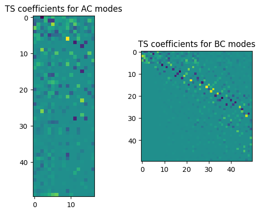
Whenever we subtract a system, we must use care that we do not subtract “too much”. A final assembly with negative mass or negative stiffness can result in issues in subsequent calculations. We will therefore examine the modes of Systems AC and BC to try to understand which modes of System C are active in those shapes. This can help inform how many modes should be kept in the reduced-order model of of System C. We will construct a modal filter using the System C shapes to solve for the modal coefficients of System C active in the mode shapes of Systems AC and BC. We collect CoordinateArray objects containing the degrees of freedom in System C, as well as the equivalent degrees of freedom in AC and BC using map_coordinate. Then, by indexing the ShapeArray objects from eigensolution with the CoordinateArray objects, we obtain the shape matrices at those degrees of freedom. We then perform the modal filtering with those shape matrices and plot the results.
[33]:
# Select degrees of freedom
constraint_dofs_c = sdpy.coordinate_array(geo['c'].node.id,['X+','Y+','Z+'],force_broadcast=True)
constraint_dofs_bc = geo['c'].map_coordinate(constraint_dofs_c,geo['bc'],node_map='position')
constraint_dofs_ac = geo['c'].map_coordinate(constraint_dofs_c,geo['ac'],node_map='position')
# Extract shape matrices
shape_matrix_c = sys['c'].eigensolution(num_modes)[constraint_dofs_c].T
shape_matrix_bc = sys['bc'].eigensolution(num_modes)[constraint_dofs_bc].T
shape_matrix_ac = sys['ac'].eigensolution(num_modes)[constraint_dofs_ac].T
# Perform the modal filter
modal_coefficients_bc = np.linalg.pinv(shape_matrix_c)@shape_matrix_bc
modal_coefficients_ac = np.linalg.pinv(shape_matrix_c)@shape_matrix_ac
# Plot the results
fig,ax = plt.subplots(1,2)
ax[0].imshow(modal_coefficients_ac)
ax[1].imshow(modal_coefficients_bc)
ax[0].set_title('TS coefficients for AC modes')
ax[1].set_title('TS coefficients for BC modes')
[33]:
Text(0.5, 1.0, 'TS coefficients for BC modes')
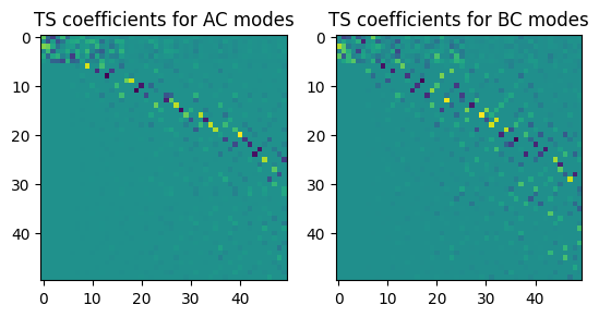
From the previous figure, we see we will need to use about 30 modes of system C to cover 50 modes of Systems AC and BC. Therefore, we will construct reduced-order models of these systems containing those modes.
[34]:
num_modes_bc = 50
num_modes_ac = 50
num_modes_c = 30
num_constraint_shapes = 30
modal_system_ac = sys['ac'].eigensolution(num_modes_ac).system()
modal_system_bc = sys['bc'].eigensolution(num_modes_bc).system()
modal_system_c = sys['c'].eigensolution(num_modes_c).system()
When we concatenate the System objects together, we will note the negative sign on modal_system_c to signify the removal of that system.
[35]:
combined_system = sdpy.System.concatenate((modal_system_ac,modal_system_bc,-modal_system_c),
node_offset)
Now we will construct the ShapeArray to use in the constraint shapes. This set of shapes must contain the mode shapes of System C at the C degrees of freedom, but also at the AC and BC degrees of freedom that overlap System C. We have already extracted these degrees of freedom, so we only need to extract the shape coefficients. We will solve for the mode shapes using the eigensolution method, extract the shape coefficients at each degree of freedom by indexing by the CoordinateArray, and then create the full shape matrix by repeating the shape matrix three times, once each for System AC, BC, and C. The final ShapeArray is constructed by combining this shape matrix with the degrees of freedom, recognizing we need to apply the node offset obtained when combining the geometries.
[36]:
# Get the mode shapes
shapes_c = modal_system_c.eigensolution(num_constraint_shapes)
# Extract shape coefficients at the requested degrees of freedom
shape_matrix = shapes_c[constraint_dofs_c]
# The full matrix will repeat this matrix 3x
full_shape_matrix = np.concatenate((shape_matrix,shape_matrix,shape_matrix),axis=-1)
# Apply the node offsets to our lists of constraint degrees of freedom
constraint_dofs_ac.node = constraint_dofs_ac.node + node_offset
constraint_dofs_bc.node = constraint_dofs_bc.node + 2*node_offset
constraint_dofs_c.node = constraint_dofs_c.node + 3*node_offset
# Assemble degrees of freedom into one list
constraint_dofs = np.concatenate([constraint_dofs_ac,constraint_dofs_bc,
constraint_dofs_c])
# Construct the constraint shapes.
constraint_shapes = sdpy.shape_array(
constraint_dofs,full_shape_matrix)
If we plot the constraint shapes on the combined geometry, we should see the System C portion of all three substructures moving in the mode shapes of System C. SDynPy makes it easy to verify that we’ve set up the constraint shapes correctly by plotting the shapes.
[37]:
combined_geometry.plot_shape(constraint_shapes,undeformed_opacity=0,deformed_opacity=0.25)
Node 10001 not found in shape array
...
Node 21100 not found in shape array
[37]:
<sdynpy.core.sdynpy_geometry.ShapePlotter at 0x1f76fb4fbf0>

Now we can apply the constraints to the system. Since we are applying constraints in two steps, we will take a slightly different approach in this case. We will still use the substructure_by_shape method; however, instead of having the method return a constrained system, we will simply have it return the constraint matrix $mathbf{B}$ by passing the keyword argument return_constrained_system=False. After we construct the constraint matrices for both sets of constraints, we will concatenate the matrices together into one constraint matrix and apply it to the system using the constrain method.
[38]:
# Create the constraint matrix between AC and C
constraint_matrix_ac_c = combined_system.substructure_by_shape(
constraint_shapes,
constraint_dofs_ac,
constraint_dofs_c,
return_constrained_system=False)
# Create the constraint matrix between BC and C
constraint_matrix_bc_c = combined_system.substructure_by_shape(
constraint_shapes,
constraint_dofs_bc,
constraint_dofs_c,
return_constrained_system=False)
# Stack the constraint matrices into a single constraint matrix
constraint_matrix = np.concatenate((constraint_matrix_ac_c,constraint_matrix_bc_c),axis=0)
# Apply the constraints to the system
constrained_system = combined_system.constrain(constraint_matrix)
# Compare results
constrained_shapes = constrained_system.eigensolution(num_modes)
comparison_plotter, mac_ax, latex_table = compare_to_truth('Case 6', geo['abc'], shp['abc'],
combined_geometry, constrained_shapes)
Case 6 Results:
Mode Freq 1 (Hz) Freq 2 (Hz) Freq Error MAC
1 463.95 463.46 0.1% 100
2 584.56 585.95 -0.2% 100
3 748.59 750.96 -0.3% 100
4 833.86 834.17 -0.0% 100
5 1367.79 1368.49 -0.1% 100
6 1440.92 1434.50 0.4% 100
7 1463.11 1458.50 0.3% 100
8 1663.66 1665.14 -0.1% 100
9 1725.24 1727.17 -0.1% 100
10 2049.77 2021.03 1.4% 100
11 2873.85 2766.90 3.9% 99
12 3142.64 3138.37 0.1% 100
13 3436.96 3432.29 0.1% 100
14 3767.00 3765.91 0.0% 100
15 3871.88 3870.86 0.0% 100
16 4107.97 4062.56 1.1% 94
17 4254.27 4250.85 0.1% 100
18 4396.10 4312.22 1.9% 94
19 4331.83 4319.28 0.3% 100
20 4978.92 4947.56 0.6% 100
21 5236.66 5193.05 0.8% 99
22 5693.47 5687.49 0.1% 100
23 6202.10 6198.35 0.1% 100
24 6225.05 6210.73 0.2% 100
25 6954.05 6945.25 0.1% 100
26 7111.83 7102.79 0.1% 100
27 7254.51 7246.99 0.1% 98
28 7357.03 7397.53 -0.5% 98
29 7833.96 7729.57 1.4% 95
30 8011.24 7992.09 0.2% 99
31 8077.55 8049.50 0.3% 97
32 8319.80 8310.52 0.1% 96
33 8851.40 8860.38 -0.1% 94
34 9438.63 9069.66 4.1% 78
35 9273.33 9263.32 0.1% 98
36 9594.14 9591.93 0.0% 99
37 9922.72 9875.70 0.5% 94
38 10161.09 10060.16 1.0% 58
39 10161.09 10307.29 -1.4% 42
40 10372.64 10369.17 0.0% 100
41 10770.20 10758.10 0.1% 98
42 11576.56 11618.55 -0.4% 98
43 11854.72 11800.98 0.5% 94
44 12132.94 12079.93 0.4% 98
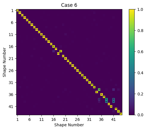

We can see we obtain very accurate results in this case, with good mode shape agreement and most frequency errors less than 1%.
Case 7: Constrain an Experimental Modal Representation of System AC to an Analytical Modal Representation of System BC and Subtract off an Analytical Modal Representation of System C
The final case examined in this paper is an example of Experimental-to-Analytical substructuring using the same Systems as Case 6. In this case, we assume System AC was measured experimentally; it has a much sparser instrumentation set of 20 triaxial sensors and a limited bandwidth up to 4000 Hz. We assume as before that we have analytical models of System BC and the transmission simulator C.
We will begin this case by transforming the analytic System AC into an experimental equivalent. We solve for the modes up to 4000 Hz, and we use effective independence with the optimize_degrees_of_freedom method to select an optimal instrumentation set to distinguish these modes. Once we have these sensors, we will reduce the System AC geometry to only these sensor locations and add tracelines to improve visualization of the experimental geometry. We will also renumber the nodes in the model, as typically an experimental modal test would use easier-to-remember node numbers than exist in a finite element model. We plot the experimental shapes on the Geometry to verify correct setup.
[39]:
# Set the number of sensors to keep
num_triax_sensors = 20
# Compute the modes the system up to 4000 Hz
modes_ac = sys['ac'].eigensolution(maximum_frequency=4000)
# Select sensor locations based on effective independence
optimal_shapes = modes_ac.optimize_degrees_of_freedom(
num_triax_sensors,group_by_node=True)
optimal_dofs = np.unique(optimal_shapes.coordinate)
test_nodes = np.unique(optimal_dofs.node)
# Reduce the analytical geometry to just the test geometry
test_geometry = geo['ac'].reduce(test_nodes)
# Connect the remaining nodes with lines for visualization
test_geometry.add_traceline(
[1,2,106,107,1,0, # 0 denotes a line break
42,118,147,42,0,
34,126,139,34,0,
1146,676,722,1126,1146,0,
1457,1472,0,
556,560,596,580,556,0,
1,42,34,0,
107,118,126,0,
106,147,139,0,
1146,556,0,
1126,580,0,
676,1457,560,0,
722,1472,596])
# Create new node numbers for the nodes in the test
node_sorting = np.argsort(test_geometry.global_node_coordinate()[:,0])[::-1]
node_map = sdpy.id_map(
test_geometry.node.id[node_sorting],
np.arange(node_sorting.size)+101)
# Map the old nodes to the new nodes in the geometry
test_geometry = test_geometry.map_ids(node_id_map=node_map)
# Map the old nodes to the new nodes in the shapes
test_shapes = optimal_shapes.copy()
test_shapes.coordinate.node = node_map(test_shapes.coordinate.node)
# Plot the shapes and label the nodes
test_geometry.plot_shape(test_shapes,plot_kwargs={'label_nodes':True})
# Create the experimental modal system
test_system = test_shapes.system()

The case then proceeds similarly to Case 6. We construct a combined geometry that will be used to visualize the results.
[40]:
combined_geometry,node_offset = sdpy.Geometry.overlay_geometries(
[test_geometry,geo['bc'],geo['c']],return_node_id_offset=True,
color_override=[1,7,11]) # Blue, Green, Red
We then investigate the mode contributions in each substructure to see how many modes should be kept in the analytical substructures. For the System BC to System C constraint, we can use all the degrees of System C.
[41]:
constraint_dofs_c_bc = sdpy.coordinate_array(geo['c'].node.id,['X+','Y+','Z+'],force_broadcast=True)
constraint_dofs_bc = geo['c'].map_coordinate(constraint_dofs_c_bc,geo['bc'],node_map='position')
However, for the test case, we will need to find the subset of the transmission simulator degrees of freedom that are in the test geometry. Here we select all of the nodes in the test with an X-coordinate less than some threshold and use map_coordinate to find the corresponding degrees of freedom.
[42]:
ac_nodes = test_geometry.node.id[test_geometry.global_node_coordinate()[:,0] < 0.062501]
constraint_dofs_ac = sdpy.coordinate_array(ac_nodes,['X+','Y+','Z+'],force_broadcast=True)
constraint_dofs_c_ac = test_geometry.map_coordinate(constraint_dofs_ac,geo['c'],node_map='position')
We can then create the shape matrices and perform the modal filtering.
[43]:
# Extract the shape matrices
shape_matrix_c_ac = sys['c'].eigensolution(num_modes)[constraint_dofs_c_ac].T
shape_matrix_c_bc = sys['c'].eigensolution(num_modes)[constraint_dofs_c_bc].T
shape_matrix_bc = sys['bc'].eigensolution(num_modes)[constraint_dofs_bc].T
shape_matrix_ac = test_system.eigensolution()[constraint_dofs_ac].T
# Compute the modal coefficients
modal_coefficients_bc = np.linalg.pinv(shape_matrix_c_bc)@shape_matrix_bc
modal_coefficients_ac = np.linalg.pinv(shape_matrix_c_ac)@shape_matrix_ac
# Plot the results
fig,ax = plt.subplots(1,2)
ax[0].imshow(modal_coefficients_ac)
ax[1].imshow(modal_coefficients_bc)
ax[0].set_title('TS coefficients for AC modes')
ax[1].set_title('TS coefficients for BC modes')
[43]:
Text(0.5, 1.0, 'TS coefficients for BC modes')
It looks like roughly 14 modes would be needed of System C to capture motions in the 16 modes of System AC up to 4000 Hz. We will also keep 25 modes of System BC. We will construct our modal systems using these modes and concatenate the systems together.
[44]:
# Select numbers of modes and create modal systems
num_modes_bc = 25
num_modes_c = 14
num_constraint_shapes = 14
modal_system_bc = sys['bc'].eigensolution(num_modes_bc).system()
modal_system_c = sys['c'].eigensolution(num_modes_c).system()
# Concatenate the systems into a single system
combined_system = sdpy.System.concatenate((test_system,modal_system_bc,-modal_system_c),
node_offset)
Now we will construct the constraint shapes, similar to Case 6. We need to build two separate shape matrices; the first matrix corresponds to the mode shapes of System C at the full analytical degrees of freedom, and the second matrix corresponds to the mode shapes of System C at just the test degrees of freedom. We have already created the CoordinateArray objects representing these degrees of freedom, so we can simply index the ShapeArray object representing the modes of System C to extract these matrices. When constructing the shapes we should remember to apply the node offsets. The constraint shapes for System BC and System C will use the full analysis set of degrees of freedom, while the constraint shapes for System AC will only use the test degrees of freedom. As always, we should plot these shapes to ensure they make sense.
[45]:
# Solve for the modes of C
shapes_c = modal_system_c.eigensolution(num_constraint_shapes)
# Extract the coefficients used in the constraints to assemble shape matrices
shape_matrix_analysis = shapes_c[constraint_dofs_c_bc]
shape_matrix_test = shapes_c[constraint_dofs_c_ac]
# Apply the node offsets for the combined geometry
constraint_dofs_ac.node = constraint_dofs_ac.node + node_offset
constraint_dofs_bc.node = constraint_dofs_bc.node + 2*node_offset
constraint_dofs_c_bc.node = constraint_dofs_c_bc.node + 3*node_offset
constraint_dofs = np.concatenate([constraint_dofs_ac,constraint_dofs_bc,
constraint_dofs_c_bc])
# Construct the full shape matrix
shape_matrix = np.concatenate([shape_matrix_test,shape_matrix_analysis,
shape_matrix_analysis],axis=-1)
# Construct the shape array
constraint_shapes = sdpy.shape_array(
constraint_dofs,shape_matrix)
# Plot the shape array
combined_geometry.plot_shape(constraint_shapes)
Node 10101 not found in shape array
...
Node 21100 not found in shape array
[45]:
<sdynpy.core.sdynpy_geometry.ShapePlotter at 0x1f756047020>

We will again use the substructure_by_shape method to return the constrain matrix \(\mathbf{B}\) by passing the keyword argument return_constrained_system=False. After we construct the constraint matrices for both sets of constraints, we will concatenate the matrices together into one constraint matrix and apply it to the system using the constrain method.
[46]:
constraint_matrix_ac_c = combined_system.substructure_by_shape(
constraint_shapes,
constraint_dofs_ac,
constraint_dofs_c_bc,
return_constrained_system=False)
constraint_matrix_bc_c = combined_system.substructure_by_shape(
constraint_shapes,
constraint_dofs_bc,
constraint_dofs_c_bc,
return_constrained_system=False)
constraint_matrix = np.concatenate((constraint_matrix_ac_c,constraint_matrix_bc_c),axis=0)
constrained_system = combined_system.constrain(constraint_matrix)
# Compare results
constrained_shapes = constrained_system.eigensolution()
comparison_plotter, mac_ax, latex_table = compare_to_truth('Case 7', geo['abc'], shp['abc'],
combined_geometry, constrained_shapes)
Case 7 Results:
Mode Freq 1 (Hz) Freq 2 (Hz) Freq Error MAC
1 464.71 463.46 0.3% 100
2 594.46 585.95 1.5% 100
3 760.13 750.96 1.2% 100
4 827.97 834.17 -0.7% 100
5 1383.69 1368.49 1.1% 100
6 1432.82 1434.50 -0.1% 99
7 1641.68 1458.50 12.6% 85
8 1825.23 1458.50 25.1% 80
9 1680.84 1665.14 0.9% 100
10 1825.23 1727.17 5.7% 60
11 2085.36 2021.03 3.2% 99
12 3276.98 2766.90 18.4% 86
13 3185.57 3138.37 1.5% 98
14 4295.96 3138.37 36.9% 42
15 3688.98 3432.29 7.5% 95
16 3697.41 3765.91 -1.8% 89
17 3891.54 3870.86 0.5% 90
18 4197.73 4062.56 3.3% 79
19 3185.57 4250.85 -25.1% 46
20 4295.96 4250.85 1.1% 98
21 4197.73 4312.22 -2.7% 90
22 6076.43 4947.56 22.8% 58
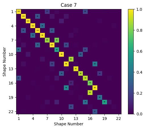

We see reasonably good results from this substructuring example. As always with Experimental-to-Analytical substructuring, the limited bandwidth of the experimental substructure will often result in errors due to modal truncation. The low frequency modes are often captured very well, while higher frequency modes show increased errors.
Conclusions
SDynPy provides a consistent framework to perform structural dynamics analyses using the Python programming language. It provides core data classes that mirror common data types found in structural dynamics. These objects have the capability to simplify performing complex structural dynamics analyses by keeping track of geometry, transformations, and degrees of freedom. SDynPy contains readers for common file types, state-of-the-art mode fitters to perform experimental modal analysis, and high-quality interactive data visualization tools. The author hopes the release of this tool will encourage the growth of open-source software in structural dynamics by providing a common framework in which users can work.