RobustWorkflow¶

This tutorial follows the robust_workflow notebook and demonstrates the RobustWorkflow class. The workflow can process data streams that are not cleanly stationary: with operate_safe=False it will, when needed, drop an initial fraction of the stream to find a stationary tail and return “ball-park” statistics (flagged in the result metadata) rather than aborting.

For each signal the procedure is the same as in the notebook:

build / load the signal into a DataStream,
set up RobustWorkflow(operate_safe=False, verbosity=2) (high verbosity so the intermediate steps are plotted),
plot the raw signal with plot_signal_basic_stats(),
call process_data_stream to get the statistics, and
re-plot the signal with its mean, confidence interval, and SSS start.

For clean single traces the DataStream Class guide is simpler; for many runs see Ensemble Analysis. RobustWorkflow assumes equally spaced time points.

Setup¶

RobustWorkflow displays its plots (it calls plt.show() and then closes the figure). The small keep_figures helper keeps those figures open just long enough for the documentation gallery to capture the workflow’s own output – it is not needed in a notebook or script.

import contextlib
import pprint
from pathlib import Path

import matplotlib.pyplot as plt
import numpy as np
import pandas as pd

import quends as qnds

plotter = qnds.Plotter()


def example_data_dir() -> Path:
    """Find the shared example data directory during script or gallery runs."""
    starts = []
    if "__file__" in globals():
        starts.append(Path(__file__).resolve())
    starts.append(Path.cwd().resolve())

    for start in starts:
        for parent in [start, *start.parents]:
            for candidate in (parent / "examples" / "data", parent / "data"):
                if candidate.is_dir():
                    return candidate
    raise FileNotFoundError("Could not locate examples/data")


DATA_DIR = example_data_dir()


@contextlib.contextmanager
def keep_figures():
    _close = plt.close
    plt.close = lambda *a, **k: None
    try:
        yield
    finally:
        plt.close = _close

Synthetic data: linear transient to a plateau with some noise¶

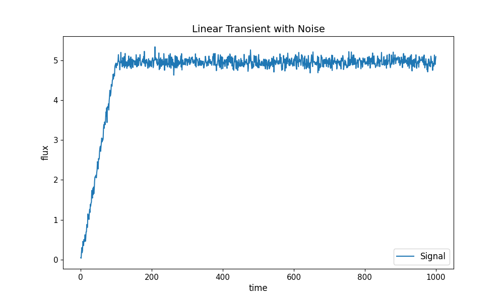
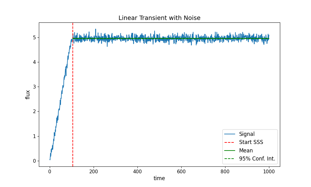
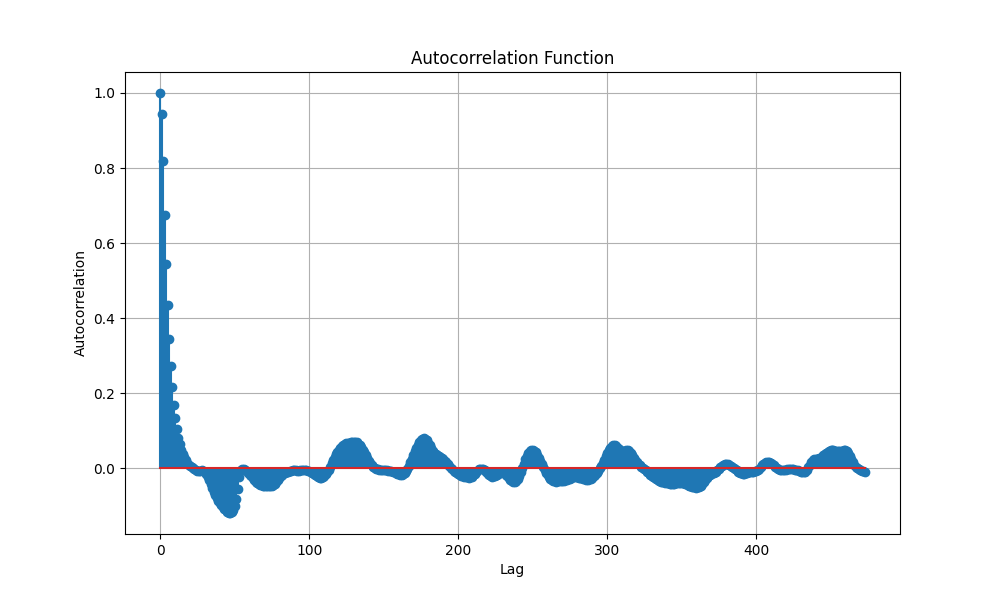
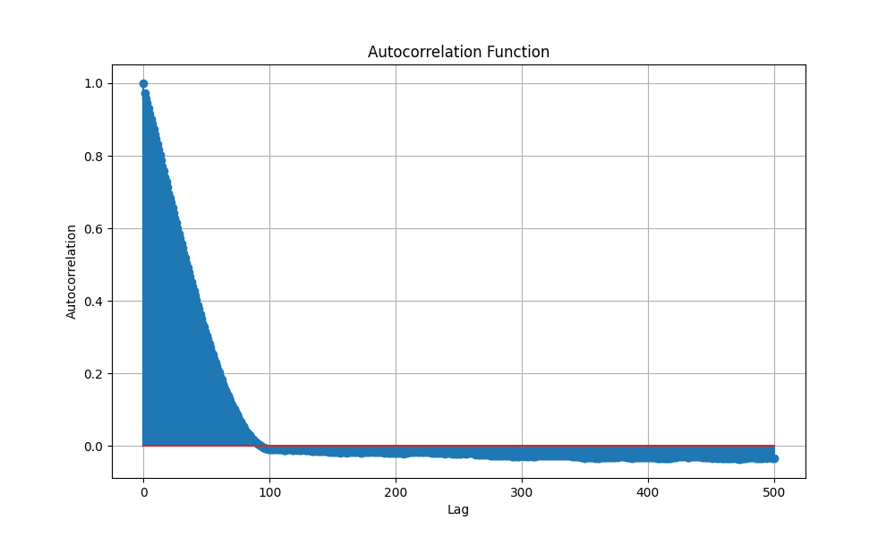
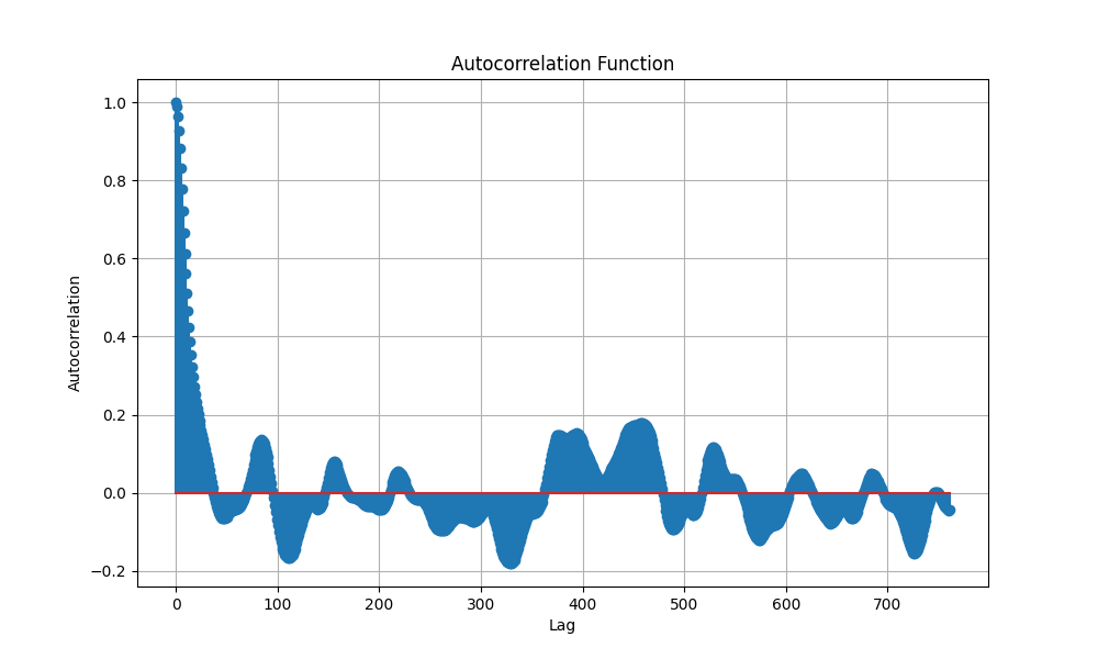
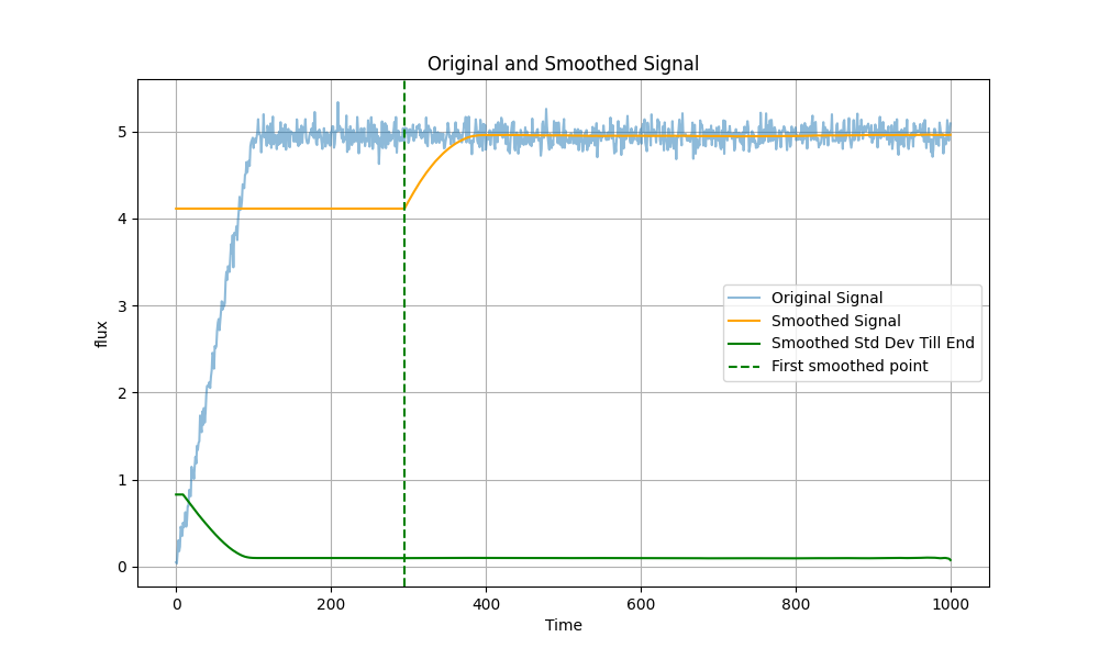
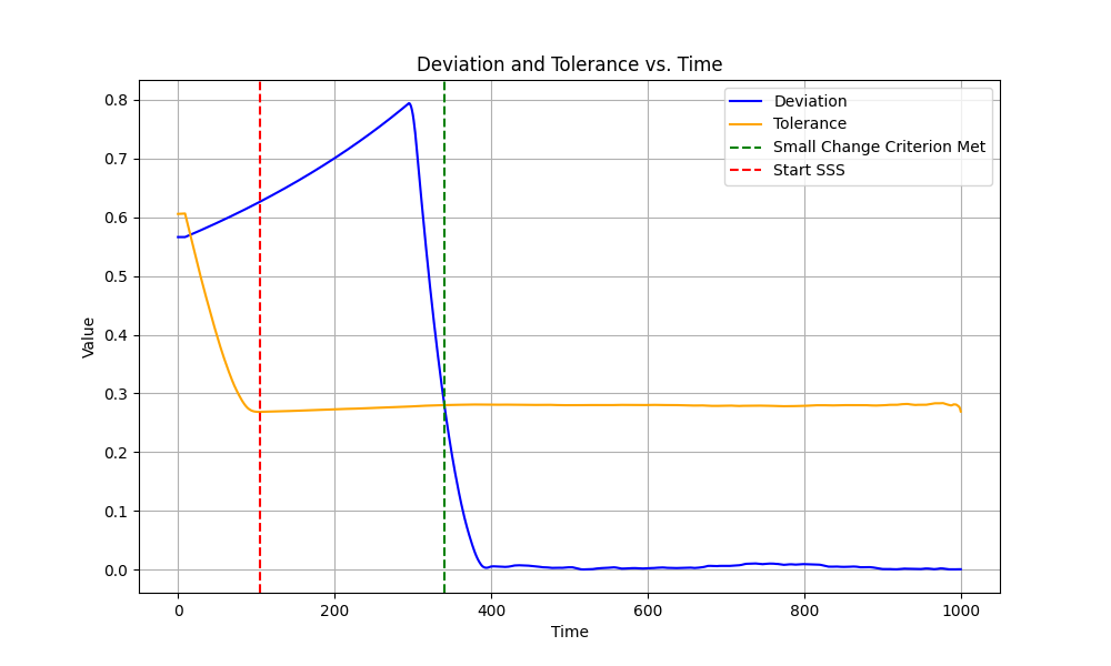
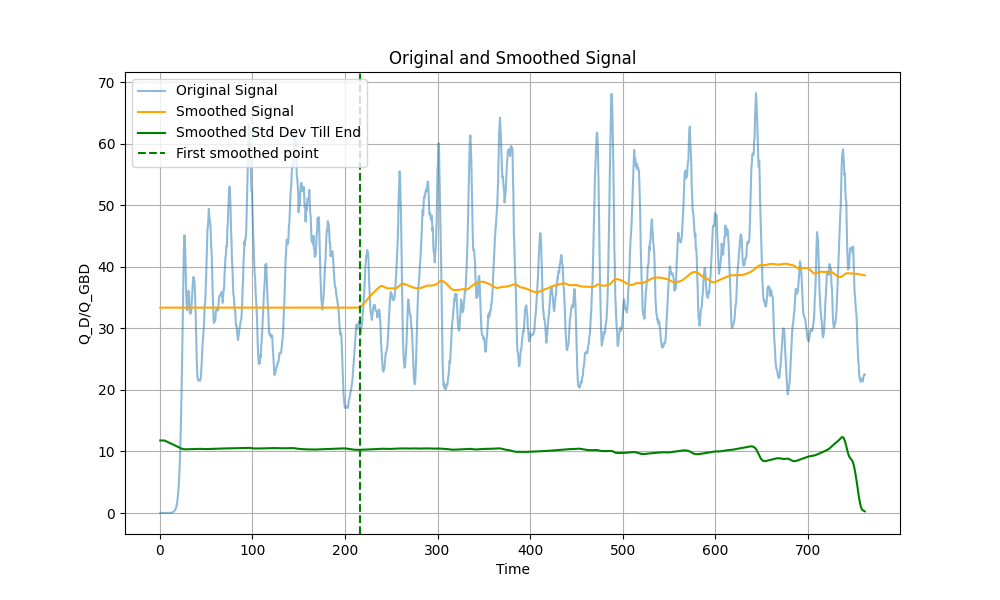
A linear ramp into a flat signal, plus noise. With verbosity=2 the workflow shows its intermediate steps: the raw signal, the autocorrelation used to set the averaging window, and the smoothed signal with the detected start of statistical steady state (SSS).

arr_time = np.linspace(start=0, stop=1000, num=1001)
arr_signal = np.zeros_like(arr_time)
n_pts = arr_signal.shape[0]
for i_arr in range(100):
    arr_signal[i_arr] = 0.05 * arr_time[i_arr]
for i_arr in range(100, n_pts):
    arr_signal[i_arr] = arr_signal[99]
np.random.seed(42)
arr_signal += np.random.normal(loc=0.0, scale=0.1, size=arr_signal.shape)

my_label = "Linear Transient with Noise"
ds_flat = qnds.DataStream(pd.DataFrame({"time": arr_time, "flux": arr_signal}))
col = "flux"

my_wrkflw = qnds.RobustWorkflow(operate_safe=False, verbosity=2)
with keep_figures():
    # Plot raw signal
    plotter.plot_signal_basic_stats(ds_flat, col, label=my_label)
    # Get statistics
    my_stats = my_wrkflw.process_data_stream(ds_flat, col)
    # Plot trace with mean and start of steady state
    if not my_stats[col]["metadata"]["mitigation"] == "Drop":
        plotter.plot_signal_basic_stats(ds_flat, col, stats=my_stats, label=my_label)

Original size of data stream: 1001 points.
After enforcing start time there are 1001 points left.
stats decorrelation length 74 gives smoothing window of 296 points.
Getting start of SSS based on smoothed signal:
Index where criterion is met: 341
Rolling window: 296
time where criterion is met: 341.0
time at start of SSS (adjusted for rolling window): 104.0

The dictionary my_stats holds the numerical results; metadata reveals how the data was processed. Here mitigation: None / status: Regular means no special handling was needed.

pprint.pprint(my_stats)

{'flux': {'ci_method': 'normal',
          'confidence_interval': (4.94708601627662, 4.960092784311302),
          'confidence_level': 0.95,
          'effective_sample_size': 897,
          'ess_blocks': 178.1770846258308,
          'independence_status': 'independent',
          'independent': True,
          'ljungbox_lags': [5, 10],
          'ljungbox_pvalue': 0.9704167699780076,
          'ljungbox_pvalues': [0.9966734615909969, 0.9704167699780076],
          'mean': 4.953589400293961,
          'mean_uncertainty': 0.0033180530700721244,
          'metadata': {'mitigation': 'None', 'status': 'Regular'},
          'n_short_averages': 179,
          'pm_std': (4.950271347223889, 4.956907453364033),
          'se_effective_n': 179.0,
          'se_method': 'iid_blocks',
          'sss_start': np.float64(104.0),
          'standard_deviation': 0.04439252454491515,
          'start_time': 0.0,
          'variance': 0.001970696235470894,
          'window_size': 5}}

Regular signals: CGYRO¶

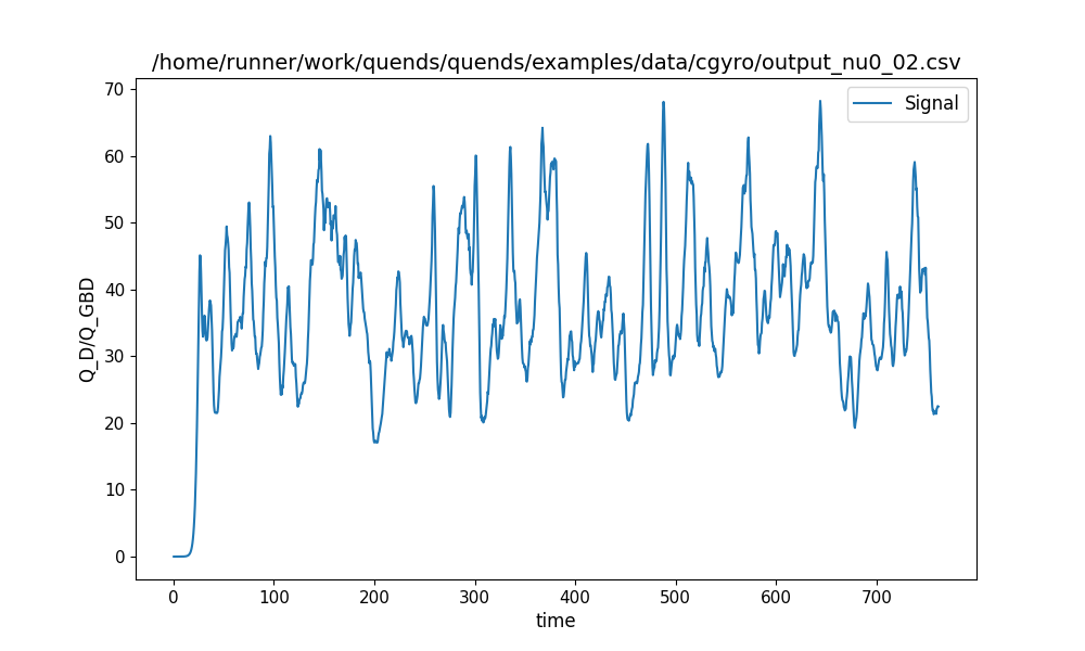
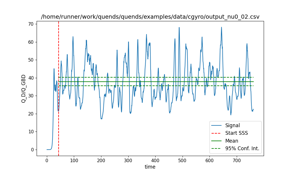
A well-behaved CGYRO run. The observable is the third column (after the index and time), exactly as in the notebook.

data_paths = [DATA_DIR / "cgyro" / "output_nu0_02.csv"]
col = pd.read_csv(data_paths[0]).columns[2]  # 3rd column (after index, time)
data_stream = qnds.from_csv(data_paths[0], col)
print("The data stream contains the following variables:")
for column, name in enumerate(data_stream.variables()):
    print(f"{column}: {name}")

my_wrkflw = qnds.RobustWorkflow(operate_safe=False, verbosity=2)
with keep_figures():
    plotter.plot_signal_basic_stats(data_stream, col, label=data_paths[0])
    my_stats = my_wrkflw.process_data_stream(data_stream, col)
    if not my_stats[col]["metadata"]["mitigation"] == "Drop":
        plotter.plot_signal_basic_stats(
            data_stream, col, stats=my_stats, label=data_paths[0]
        )

The data stream contains the following variables:
0: time
1: Q_D/Q_GBD
Original size of data stream: 1523 points.
After enforcing start time there are 1523 points left.
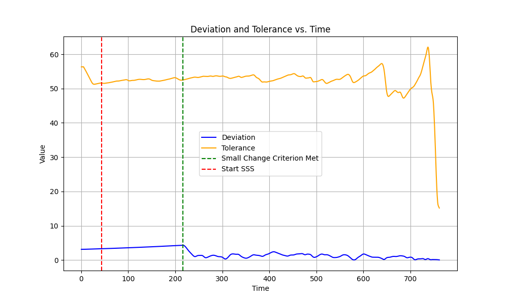
stats decorrelation length 108 gives smoothing window of 432 points.
Getting start of SSS based on smoothed signal:
Index where criterion is met: 431
Rolling window: 432
time where criterion is met: 216.0
time at start of SSS (adjusted for rolling window): 43.0

Most of this signal is in SSS: the mean is steady and its high standard deviation gives the steady-state criterion plenty of wiggle room.

pprint.pprint(my_stats)

{'Q_D/Q_GBD': {'ci_method': 'normal',
               'confidence_interval': (35.5192927099123, 40.30162589947248),
               'confidence_level': 0.95,
               'effective_sample_size': 68,
               'ess_blocks': 33.0,
               'independence_status': 'independent',
               'independent': True,
               'ljungbox_lags': [5, 10],
               'ljungbox_pvalue': 0.3238689374520419,
               'ljungbox_pvalues': [0.7837931462743449, 0.3238689374520419],
               'mean': 37.91045930469239,
               'mean_uncertainty': 1.219982956520453,
               'metadata': {'mitigation': 'None', 'status': 'Regular'},
               'n_short_averages': 33,
               'pm_std': (36.690476348171934, 39.13044226121284),
               'se_effective_n': 33.0,
               'se_method': 'iid_blocks',
               'sss_start': np.float64(43.0),
               'standard_deviation': 7.008268521440423,
               'start_time': 0.0,
               'variance': 49.115827668612724,
               'window_size': 43}}

Regular signals: GX¶

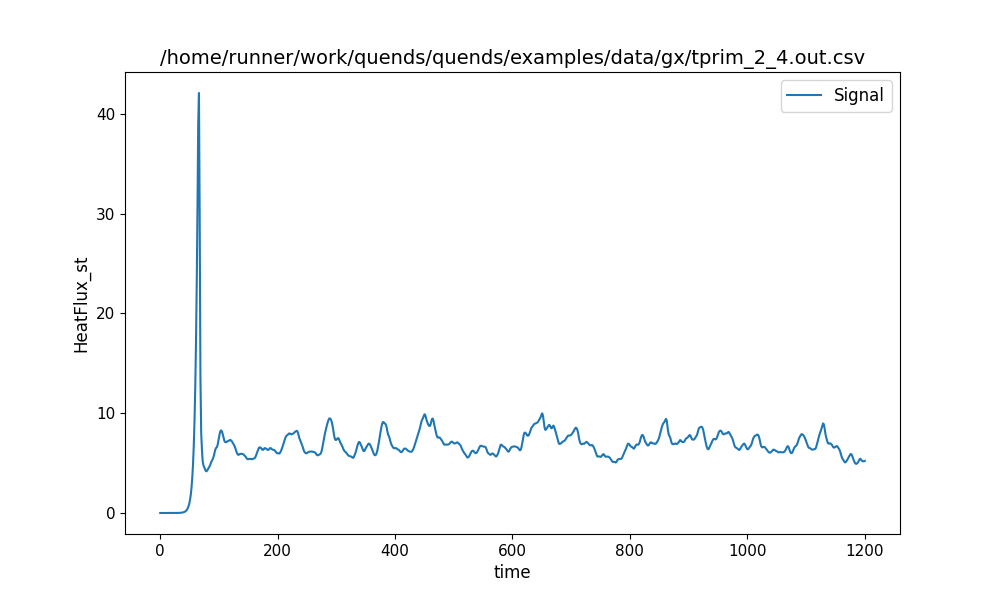
A GX heat-flux trace (HeatFlux_st).

data_paths = [DATA_DIR / "gx" / "tprim_2_4.out.csv"]
data_stream = qnds.from_csv(data_paths[0], "HeatFlux_st")
print("The data stream contains the following variables:")
for column, name in enumerate(data_stream.variables()):
    print(f"{column}: {name}")
col = "HeatFlux_st"

my_wrkflw = qnds.RobustWorkflow(operate_safe=False, verbosity=2)
with keep_figures():
    plotter.plot_signal_basic_stats(data_stream, col, label=data_paths[0])
    my_stats = my_wrkflw.process_data_stream(data_stream, col)
    if not my_stats[col]["metadata"]["mitigation"] == "Drop":
        plotter.plot_signal_basic_stats(
            data_stream, col, stats=my_stats, label=data_paths[0]
        )

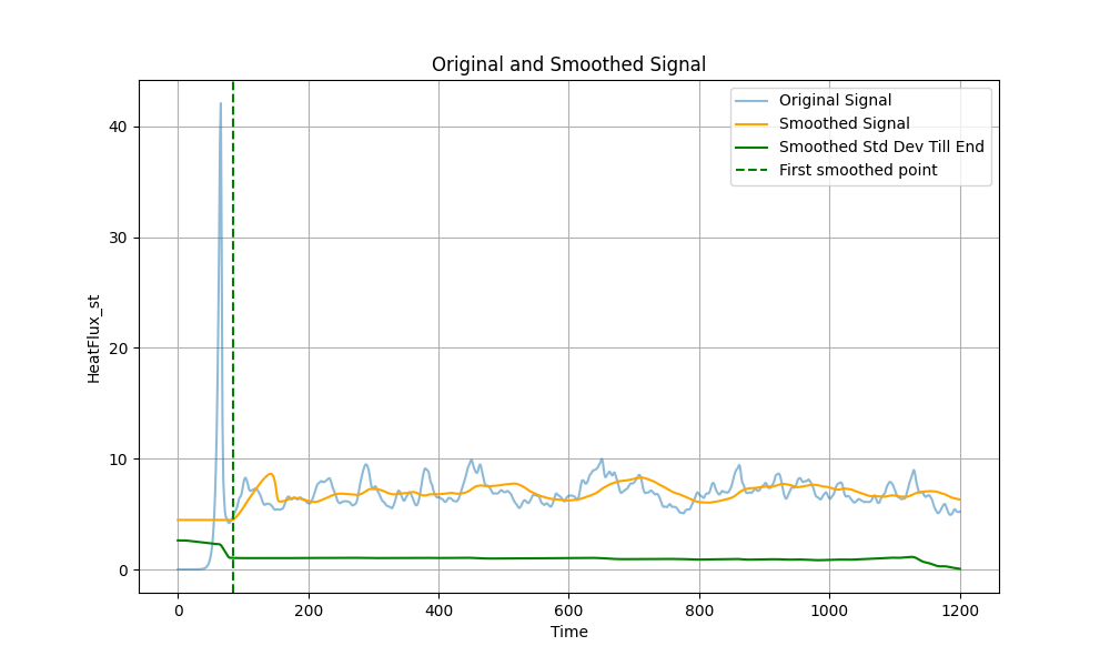
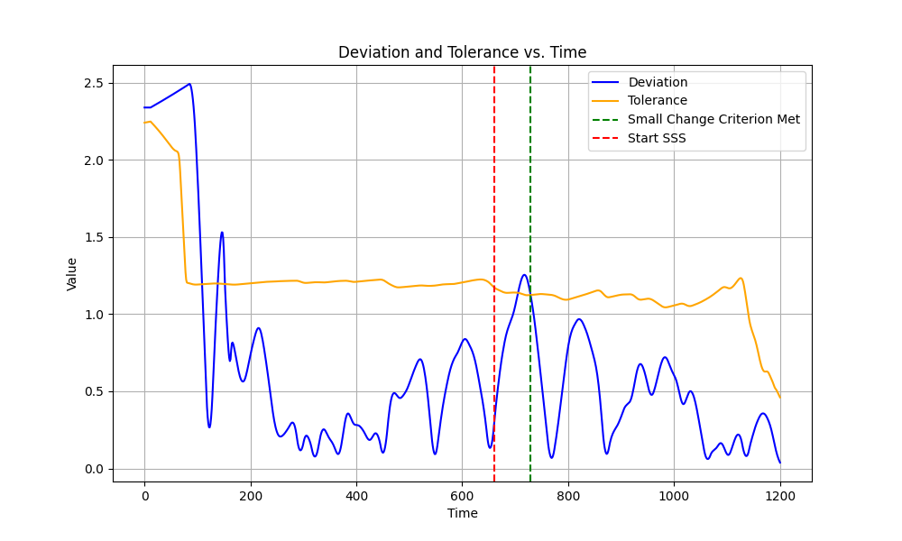
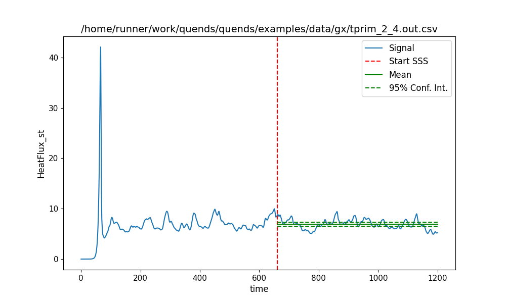
The data stream contains the following variables:
0: time
1: HeatFlux_st
Original size of data stream: 947 points.
After enforcing start time there are 947 points left.
stats decorrelation length 17 gives smoothing window of 68 points.
Getting start of SSS based on smoothed signal:
Index where criterion is met: 575
Rolling window: 68
time where criterion is met: 729.4152185935495
time at start of SSS (adjusted for rolling window): 659.6462806224445

Here the decorrelation length is short, so the smoothed signal is more variable and about half the trace is identified as steady state.

pprint.pprint(my_stats)

{'HeatFlux_st': {'ci_method': 'normal',
                 'confidence_interval': (6.551702979095916, 7.341478483285037),
                 'confidence_level': 0.95,
                 'effective_sample_size': 16,
                 'ess_blocks': 15.0,
                 'independence_status': 'independent',
                 'independent': True,
                 'ljungbox_lags': [5, 10],
                 'ljungbox_pvalue': 0.6627641836511833,
                 'ljungbox_pvalues': [0.6958443642828225, 0.6627641836511833],
                 'mean': 6.946590731190477,
                 'mean_uncertainty': 0.20147334290538818,
                 'metadata': {'mitigation': 'None', 'status': 'Regular'},
                 'n_short_averages': 15,
                 'pm_std': (6.745117388285088, 7.148064074095865),
                 'se_effective_n': 15.0,
                 'se_method': 'iid_blocks',
                 'sss_start': np.float64(659.6462806224445),
                 'standard_deviation': 0.7803029017773047,
                 'start_time': 0.0,
                 'variance': 0.608872618522082,
                 'window_size': 28}}

Total running time of the script: (0 minutes 1.847 seconds)

Gallery generated by Sphinx-Gallery

Last update: Aug 11, 2026