Ensemble Analysis¶

This tutorial analyses multiple simulation runs together with the Ensemble object, using the GX members in examples/data/gx/ensemble.

Instead of one long trace, an ensemble combines several shorter runs. QUENDS provides three ways to turn an ensemble into a mean with an honest uncertainty:

Ensemble Average – average the members onto a common grid, then analyse that single averaged trace,
Serialization (pooled block means) – pool the per-member block means,
Inverse-Variance-Weighted (IVW) – weight each member’s mean by its inverse variance.

For single-trace analysis, see the DataStream Class guide. Trim/statistics parameters follow the QUENDS paper analysis notebooks for the stellarator GX ensemble (method="threshold", window_size=50, start_time=100, threshold=0.19).

Import QUENDS

import glob
from pathlib import Path

import quends as qnds


def example_data_dir() -> Path:
    """Find the shared example data directory during script or gallery runs."""
    starts = []
    if "__file__" in globals():
        starts.append(Path(__file__).resolve())
    starts.append(Path.cwd().resolve())

    for start in starts:
        for parent in [start, *start.parents]:
            for candidate in (parent / "examples" / "data", parent / "data"):
                if candidate.is_dir():
                    return candidate
    raise FileNotFoundError("Could not locate examples/data")


COL = "HeatFlux_st"
DATA_DIR = example_data_dir()
plotter = qnds.Plotter()

Data Loading¶

Ensemble.from_files loads each CSV into a member DataStream.

gx_files = sorted(glob.glob(str(DATA_DIR / "gx" / "ensemble" / "tprim_2_5_*.out.csv")))
ens = qnds.Ensemble.from_files(gx_files, COL)
print("ensemble members:", len(ens.members()))

ensemble members: 4

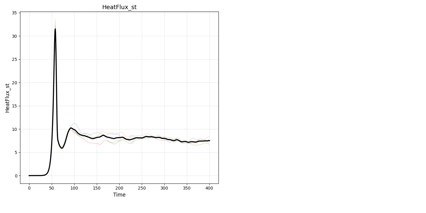
Plotting all members together with the ensemble average.

plot = plotter.plot_ensemble_with_average(
    ens, variables_to_plot=[COL], condensed_legend=True, show=True
)

Ensemble Average Approach¶

Average the members onto a common time grid, then analyse that single averaged trace exactly like a single run.

Build the averaged DataStream and check stationarity.

avg = ens.compute_average_ensemble()
print("averaged trace rows:", len(avg))
print("avg is_stationary:", avg.is_stationary(COL))

averaged trace rows: 740
avg is_stationary: {'HeatFlux_st': True}

Trim the averaged trace, then read off its ESS.

avg_trimmed = avg.trim(
    method="threshold", window_size=50, start_time=100, threshold=0.19
)
print("avg sss_start:", avg_trimmed.trim_metadata.get("sss_start"))
print("avg ESS:", avg_trimmed.effective_sample_size())

avg sss_start: 126.838088
/home/runner/work/quends/quends/src/quends/base/utils.py:300: UserWarning: The computed signal decorrelation time is large compared to the max lag in the computation of the autocorrelation. Results may be inaccurate. Estimated tau_int=116.19, nlags=126.
  warnings.warn(
avg ESS: {'results': {'HeatFlux_st': 5}}

The Ensemble Average estimate of the mean and its uncertainty. We analyse the trimmed averaged trace (average -> trim -> statistics), so the transient is removed before the mean and its standard error are computed. NB: the ensemble_average estimator does not trim internally – running it on a raw, un-trimmed average folds the transient into the variance and greatly inflates the uncertainty.

ea_stats = avg_trimmed.compute_statistics(method="non-overlapping")[COL]
print("Ensemble Average ->", ea_stats)

Ensemble Average -> {'mean': 7.94494859258104, 'mean_uncertainty': 0.12784770311653157, 'variance': 0.14710531672955518, 'confidence_interval': (7.694367094472638, 8.195530090689441), 'standard_deviation': 0.38354310934959474, 'pm_std': (7.817100889464509, 8.072796295697572), 'effective_sample_size': 5, 'window_size': 51, 'n_short_averages': 9, 'ess_blocks': 4.868431876206393, 'se_effective_n': 9.0, 'se_method': 'iid_blocks', 'independence_status': 'independent', 'independent': True, 'ljungbox_lags': [5, 8], 'ljungbox_pvalues': [0.628211818690967, 0.09060661184104132], 'ljungbox_pvalue': 0.09060661184104132, 'ci_method': 'normal', 'confidence_level': 0.95, 'metadata': {'warnings': ['The computed signal decorrelation time is large compared to the max lag in the computation of the autocorrelation. Results may be inaccurate. Estimated tau_int=116.19, nlags=126.']}}

Serialization (Pooled Block Means) Approach¶

Rather than averaging the traces, pool the per-member block means. Trim every member first, then aggregate across members.

ens_trimmed = ens.trim(
    column_name=COL, method="threshold", window_size=50, start_time=100, threshold=0.19
)
print("members stationary:", ens.is_stationary(COL)["results"])
print("ESS (pooled_block_means):", ens_trimmed.effective_sample_size(COL)["results"])

members stationary: {'Member 0': {'HeatFlux_st': True}, 'Member 1': {'HeatFlux_st': True}, 'Member 2': {'HeatFlux_st': True}, 'Member 3': {'HeatFlux_st': True}}
/home/runner/work/quends/quends/src/quends/base/utils.py:300: UserWarning: The computed signal decorrelation time is large compared to the max lag in the computation of the autocorrelation. Results may be inaccurate. Estimated tau_int=20.34, nlags=25.
  warnings.warn(
/home/runner/work/quends/quends/src/quends/base/utils.py:300: UserWarning: The computed signal decorrelation time is large compared to the max lag in the computation of the autocorrelation. Results may be inaccurate. Estimated tau_int=28.08, nlags=25.
  warnings.warn(
/home/runner/work/quends/quends/src/quends/base/utils.py:300: UserWarning: The computed signal decorrelation time is large compared to the max lag in the computation of the autocorrelation. Results may be inaccurate. Estimated tau_int=24.56, nlags=18.
  warnings.warn(
/home/runner/work/quends/quends/src/quends/base/utils.py:300: UserWarning: The computed signal decorrelation time is large compared to the max lag in the computation of the autocorrelation. Results may be inaccurate. Estimated tau_int=15.30, nlags=24.
  warnings.warn(
ESS (pooled_block_means): {'HeatFlux_st': 13.164635042137682}

The serialization estimate of the mean and its uncertainty, on the trimmed members.

ser_stats = ens_trimmed.compute_uncertainty(
    method="pooled_block_means", column_name=COL
)["results"][COL]
print("Serialization ->", ser_stats)

Serialization -> {'mean': 7.796421158767362, 'variance': 0.3107674364166239, 'ess_blocks': 13.164635042137682, 'n_short_averages': 32, 'mean_uncertainty': 0.15364319888420833, 'mean_uncertainty_sem_n': 0.09854685377027263, 'mean_uncertainty_sem_ess': 0.15364319888420833, 'se_method': 'sem_ess (members_not_all_independent)', 'warning': 'Some members used best_p window. Not all members passed independence; using ESS-based SEM.', 'confidence_interval': (7.4952804889543145, 8.09756182858041), 'pm_std': (7.642777959883154, 7.950064357651571), 'window_size': 12, 'member_window_sizes': [12, 12, 9, 12], 'window_size_summary': 12, 'window_size_summary_method': 'median', 'window_size_min': 9, 'window_size_max': 12, 'independent': False, 'independence_status': 'some_independent', 'ljungbox_pvalue': 0.0021946248310642496, 'ljungbox_pvalues': [0.05617425200409796, 0.004476994141746214, 0.0021946248310642496, 0.13347036331480538], 'ljungbox_lags': [5, 5, 5, 5], 'ci_method': 'normal', 'confidence_level': 0.95, 'member_all_independent': False, 'member_some_best_p': True}

Inverse-Variance-Weighted (IVW) Approach¶

Combine the per-member means weighting each by its inverse variance, so better-resolved members count more. Trimming/stationarity are as above.

print("ESS (ivw):", ens_trimmed.effective_sample_size(COL, technique="ivw")["results"])
ivw_stats = ens_trimmed.compute_uncertainty(method="ivw", column_name=COL)["results"][
    COL
]
print("IVW ->", ivw_stats)

ESS (ivw): {'HeatFlux_st': 20.5090946620309}
IVW -> {'mean': 7.783719757167311, 'mean_uncertainty': 0.07425546570409433, 'confidence_interval': (7.638179044387286, 7.9292604699473355), 'pm_std': (7.709464291463217, 7.857975222871405), 'variance': 0.309226765823394, 'ess_blocks': 20.5090946620309, 'n_short_averages': 34.0, 'se_method': 'ivw_member_means', 'warning': None, 'window_size': 12, 'member_window_sizes': [10, 17, 13, 7], 'window_size_summary': 12, 'window_size_summary_method': 'median', 'window_size_min': 7, 'window_size_max': 17, 'independence_status': 'all_independent', 'independent': True, 'ljungbox_pvalue': 0.06735850513592934, 'ljungbox_pvalues': [0.05675964391256825, 0.05366281164550079, 0.08459568298330894, 0.07441588200233934], 'ljungbox_lags': [5, 9], 'ci_method': 'normal', 'confidence_level': 0.95, 'individual': None}

Computed on the trimmed steady-state data, the three approaches give consistent means with comparable uncertainties – a useful cross-check on an ensemble.

for name, r in [
    ("Ensemble Average", ea_stats),
    ("Serialization", ser_stats),
    ("IVW", ivw_stats),
]:
    print(
        f"{name:18s} mean={r.get('mean'):.4f}  uncertainty={r.get('uncertainty', r.get('mean_uncertainty')):.4f}"
    )

Ensemble Average   mean=7.9449  uncertainty=0.1278
Serialization      mean=7.7964  uncertainty=0.1536
IVW                mean=7.7837  uncertainty=0.0743

Total running time of the script: (0 minutes 0.335 seconds)

Gallery generated by Sphinx-Gallery

Last update: Aug 11, 2026