Note
Go to the end to download the full example code.
DataStream Class#
This tutorial demonstrates the usage of the DataStream class, which provides methods for analyzing time-series data.
- The following features are:
Trimming: Identifies steady-state regions in data.
Statistical Analysis: Computes mean, standard deviation, confidence intervals, and cumulative statistics.
Stationarity Testing: Uses the Augmented Dickey-Fuller test.
Effective Sample Size (ESS): Estimates the independent sample size.
Optimal Window Size: Determines the best window for data smoothing.
Import DataStream
import quends as qnds
GX Data Analysis#
Analysis on GX Data
# Specify the file paths
csv_file_path = "gx/tprim_2_0.out.csv"
csv2_file_path = "gx/ensemble/tprim_2_5_a.out.csv"

# Load the data from CSV files
data_stream_csv = qnds.from_csv(csv_file_path)
data_stream_gx = qnds.from_csv(csv2_file_path)

# Display the first few rows of the GX data
data_stream_gx.head()
Get available variables
data_stream_gx.variables()
Index(['time', 'Phi2_t', 'Phi2_kxt', 'Phi2_kyt', 'Phi2_kxkyt', 'Phi2_zt',
       'Apar2_t', 'Apar2_kxt', 'Apar2_kyt', 'Apar2_kxkyt', 'Apar2_zt',
       'Phi2_zonal_t', 'Phi2_zonal_kxt', 'Phi2_zonal_zt', 'Wg_st', 'Wg_kxst',
       'Wg_kyst', 'Wg_kxkyst', 'Wg_zst', 'Wg_lmst', 'Wphi_st', 'Wphi_kxst',
       'Wphi_kyst', 'Wphi_kxkyst', 'Wphi_zst', 'Wapar_st', 'Wapar_kxst',
       'Wapar_kyst', 'Wapar_kxkyst', 'Wapar_zst', 'HeatFlux_st',
       'HeatFlux_kxst', 'HeatFlux_kyst', 'HeatFlux_kxkyst', 'HeatFlux_zst',
       'HeatFluxES_st', 'HeatFluxES_kxst', 'HeatFluxES_kyst',
       'HeatFluxES_kxkyst', 'HeatFluxES_zst', 'HeatFluxApar_st',
       'HeatFluxApar_kxst', 'HeatFluxApar_kyst', 'HeatFluxApar_kxkyst',
       'HeatFluxApar_zst', 'HeatFluxBpar_st', 'HeatFluxBpar_kxst',
       'HeatFluxBpar_kyst', 'HeatFluxBpar_kxkyst', 'HeatFluxBpar_zst',
       'ParticleFlux_st', 'ParticleFlux_kxst', 'ParticleFlux_kyst',
       'ParticleFlux_kxkyst', 'ParticleFlux_zst', 'TurbulentHeating_st',
       'TurbulentHeating_kxst', 'TurbulentHeating_kyst',
       'TurbulentHeating_kxkyst', 'TurbulentHeating_zst'],
      dtype='object')
Get number of rows from the following data in GX
len(data_stream_gx)
201
Stationary Check#
# Check if a single column is stationary
data_stream_gx.is_stationary("HeatFlux_st")

# Check if multiple columns are stationary
data_stream_gx.is_stationary(["HeatFlux_st", "Wg_st", "Phi2_t"])
{'HeatFlux_st': True, 'Wg_st': True, 'Phi2_t': False}
Trimming data based to obtain steady-state portion#
Trim the data based on standard deviation method
# Returns: Dictionary with keys like "results" and "metadata"
trimmed = data_stream_gx.trim(column_name="HeatFlux_st", batch_size=50, method="std")

# Print first 5 rows of dataframe
trimmed.head()
Trim the data based on rolling variance method
trimmed = data_stream_gx.trim(
    column_name="HeatFlux_st", batch_size=50, method="rolling_variance", threshold=0.10
)

# Gather results
trimmed.head()
Trim the data based on threshold method
trimmed = data_stream_gx.trim(
    column_name="HeatFlux_st", batch_size=50, method="threshold", threshold=0.1
)

# View trimmed data
trimmed.head()
Effective Sample Size#
Compute Effective Sample Size for specific columns in GX
ess_dict = data_stream_gx.effective_sample_size(column_names=["HeatFlux_st", "Wg_st"])
print(ess_dict)
{'results': {'HeatFlux_st': 24, 'Wg_st': 10}, 'metadata': [{'operation': 'is_stationary', 'options': {'columns': 'HeatFlux_st'}}, {'operation': 'effective_sample_size', 'options': {'column_names': ['HeatFlux_st', 'Wg_st'], 'alpha': 0.05}}]}
Compute Effective sample size for trimmed data
ess_df = trimmed.effective_sample_size()
print(ess_df)
{'results': {'HeatFlux_st': 5}, 'metadata': [{'operation': 'is_stationary', 'options': {'columns': 'HeatFlux_st'}}, {'operation': 'trim', 'options': {'column_name': 'HeatFlux_st', 'batch_size': 50, 'start_time': 0.0, 'method': 'threshold', 'threshold': 0.1, 'robust': True, 'sss_start': 158.59277222661015}}, {'operation': 'effective_sample_size', 'options': {'column_names': None, 'alpha': 0.05}}]}
UQ Analysis#
Compute Statistics on trimmed dataframe
stats = trimmed.compute_statistics(method="sliding")
print(stats)

stats_df = stats["HeatFlux_st"]
{'HeatFlux_st': {'mean': 7.9406914994528615, 'mean_uncertainty': 0.08981775761011032, 'confidence_interval': (7.764648694537045, 8.116734304368677), 'pm_std': (7.850873741842751, 8.030509257062972), 'effective_sample_size': 5, 'window_size': 24}, 'metadata': [{'operation': 'is_stationary', 'options': {'columns': 'HeatFlux_st'}}, {'operation': 'trim', 'options': {'column_name': 'HeatFlux_st', 'batch_size': 50, 'start_time': 0.0, 'method': 'threshold', 'threshold': 0.1, 'robust': True, 'sss_start': 158.59277222661015}}, {'operation': 'effective_sample_size', 'options': {'column_names': None, 'alpha': 0.05}}, {'operation': 'compute_statistics', 'options': {'column_name': None, 'ddof': 1, 'method': 'sliding', 'window_size': None}}]}
Exporter Below Displays the information as a DataFrame
exporter = qnds.Exporter()
exporter.display_dataframe(stats_df)
       mean  mean_uncertainty  ...  effective_sample_size  window_size
0  7.940691          0.089818  ...                      5           24
1  7.940691          0.089818  ...                      5           24

[2 rows x 6 columns]
Below Displays the information in JSON
exporter.display_json(stats_df)
{
  "mean": 7.9406914994528615,
  "mean_uncertainty": 0.08981775761011032,
  "confidence_interval": [
    7.764648694537045,
    8.116734304368677
  ],
  "pm_std": [
    7.850873741842751,
    8.030509257062972
  ],
  "effective_sample_size": 5,
  "window_size": 24
}
Other statistical methods#
Calculate the mean with a window size of 10
mean_df = trimmed.mean(window_size=10)
print(mean_df)
{'HeatFlux_st': 7.989677796666666}
Calculate the mean with the method of sliding
mean_df = trimmed.mean(method="sliding")
print(mean_df)
{'HeatFlux_st': 7.9406914994528615}
Calculate the mean uncertainty
uq_df = trimmed.mean_uncertainty()
print(uq_df)
{'HeatFlux_st': 0.23525686516667507}
Calculate the mean uncertainty with the method of sliding
uq_df = trimmed.mean_uncertainty(method="sliding")
uq_df
{'HeatFlux_st': 0.08981775761011032}
Calculate the confidence intervale with the trimmed dataframe
ci_df = trimmed.confidence_interval()
print(ci_df)
{'HeatFlux_st': (7.528574340939983, 8.45078125239335)}
Cumlative Statistics
cumulative = trimmed.cumulative_statistics()
print(cumulative)

cumulative_df = cumulative["HeatFlux_st"]
{'HeatFlux_st': {'cumulative_mean': [8.777007562500001, 8.427817691666668, 8.308147695833334, 8.086430926041666, 7.989677796666667], 'cumulative_uncertainty': [nan, 0.4938290511758112, 0.40607424148898075, 0.553682367211838, 0.5260503426861878], 'standard_error': [nan, 0.3491898708333347, 0.23444707263463616, 0.276841183605919, 0.23525686516667502], 'window_size': 24}, 'metadata': [{'operation': 'is_stationary', 'options': {'columns': 'HeatFlux_st'}}, {'operation': 'trim', 'options': {'column_name': 'HeatFlux_st', 'batch_size': 50, 'start_time': 0.0, 'method': 'threshold', 'threshold': 0.1, 'robust': True, 'sss_start': 158.59277222661015}}, {'operation': 'effective_sample_size', 'options': {'column_names': 'HeatFlux_st', 'alpha': 0.05}}, {'operation': 'cumulative_statistics', 'options': {'column_name': None, 'method': 'non-overlapping', 'window_size': None}}]}
Display Cumulative Statistics as a DataFrame
exporter.display_dataframe(cumulative_df)
   cumulative_mean  cumulative_uncertainty  standard_error  window_size
0         8.777008                     NaN             NaN           24
1         8.427818                0.493829        0.349190           24
2         8.308148                0.406074        0.234447           24
3         8.086431                0.553682        0.276841           24
4         7.989678                0.526050        0.235257           24
CGYRO Data Analysis#
Specify the file paths
csv_file_path = "cgyro/output_nu0_50.csv"
data_stream_cg = qnds.from_csv(csv_file_path)
data_stream_cg.head()
Get the number of rows
len(data_stream_cg)
1748
Trim the data based on threshold method
trimmed_ = data_stream_cg.trim(column_name="Q_D/Q_GBD", method="std", robust=True)
# View trimmed data
print(trimmed_)
<quends.base.data_stream.DataStream object at 0x13c7ce510>
trimmed_.head()
To check if data stream is stationary
data_stream_cg.is_stationary("Q_D/Q_GBD")
{'Q_D/Q_GBD': True}
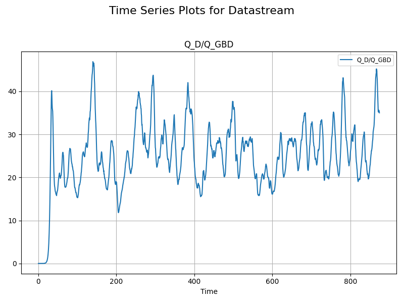
To Plot for DataStream
plotter = qnds.Plotter()
plot = plotter.trace_plot(data_stream_cg, ["Q_D/Q_GBD"])
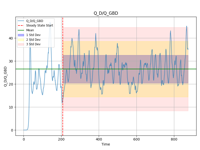
plot = plotter.steady_state_automatic_plot(
    data_stream_cg, variables_to_plot=["Q_D/Q_GBD"]
)
plot = plotter.steady_state_plot(data_stream_cg, variables_to_plot=["Q_D/Q_GBD"])
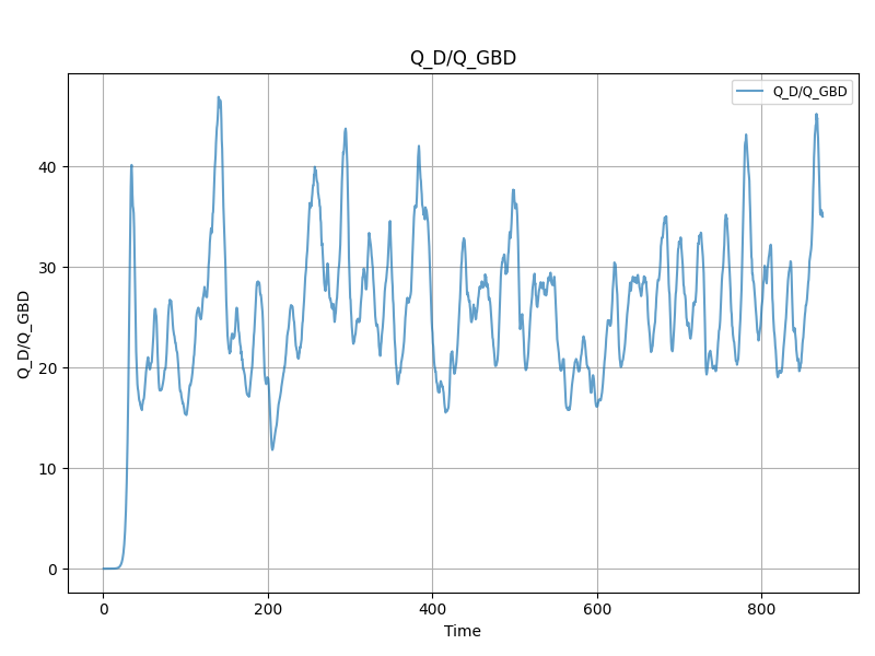
For Q_D/Q_GBD, no manual steady state start provided. Plotting raw signal.
To show additional data use:
addition_info = trimmed.additional_data(method="sliding")
print(addition_info)
{'HeatFlux_st': {'A_est': 0.03170698677588585, 'p_est': 0.5410018913986299, 'n_current': 99, 'current_sem': 0.00263944463499645, 'target_sem': 0.002375500171496805, 'n_target': 120.28580081212739, 'additional_samples': 22, 'window_size': 24}, 'metadata': [{'operation': 'is_stationary', 'options': {'columns': 'HeatFlux_st'}}, {'operation': 'trim', 'options': {'column_name': 'HeatFlux_st', 'batch_size': 50, 'start_time': 0.0, 'method': 'threshold', 'threshold': 0.1, 'robust': True, 'sss_start': 158.59277222661015}}, {'operation': 'effective_sample_size', 'options': {'column_names': 'HeatFlux_st', 'alpha': 0.05}}, {'operation': 'additional_data', 'options': {'column_name': None, 'ddof': 1, 'method': 'sliding', 'window_size': None, 'reduction_factor': 0.1}}]}
To add a reduction factor
addition_info = trimmed.additional_data(reduction_factor=0.2)
print(addition_info)
{'HeatFlux_st': {'A_est': 0.03170698677588585, 'p_est': 0.5410018913986299, 'n_current': 99, 'current_sem': 0.00263944463499645, 'target_sem': 0.00211155570799716, 'n_target': 149.54291116020593, 'additional_samples': 51, 'window_size': 24}, 'metadata': [{'operation': 'is_stationary', 'options': {'columns': 'HeatFlux_st'}}, {'operation': 'trim', 'options': {'column_name': 'HeatFlux_st', 'batch_size': 50, 'start_time': 0.0, 'method': 'threshold', 'threshold': 0.1, 'robust': True, 'sss_start': 158.59277222661015}}, {'operation': 'effective_sample_size', 'options': {'column_names': 'HeatFlux_st', 'alpha': 0.05}}, {'operation': 'additional_data', 'options': {'column_name': None, 'ddof': 1, 'method': 'sliding', 'window_size': None, 'reduction_factor': 0.2}}]}
Total running time of the script: (0 minutes 4.791 seconds)