Writing input files

Both the eig_calc.py and network_opt.py scripts take an input file that specifies the configuration for that run. Each are .dat files where each line specifies a different configuration variable.

Input for eig_calc.py

The input file for eig_cal.py is structured:

Line Number	Description	Example
Line 1	Number of synthetic events to test	32
Line 2	Number of possible events in the event space	8192
Line 3	Number of realizations of data per event	2
Line 4	Boundary information filename: JSON file containing bounds for each dimension of the event space (see Performing bounded optimization for more details)	event_bounds.json
Line 5	Path to .py file containing sampling functions and pdfs for both prior distribution and importance distribution	sample_gen.py
Line 6	Sensor 1: Lat, Long, SNR offset, Length of sensor output vec, sensor type	40.0,-111.5,0.1,2,0
Line 7	Sensor 2: Lat, Long, SNR offset, Length of sensor output vec, sensor type	41.0,-111.9,0.1,2,0
…
Line 5+N	Sensor N: Lat, Long, SNR offset, Length of sensor output vec, sensor type	40.0,-110.0,0.1,2,0

For details on the sensor options, see Sensors.

Note that for HPC simulations, the number of synthetic events to test and number of possible events in the event space must be divisible by the number of cores. For example this configuration is valid if ncores = 1,2,4,8,16, or 32. Also note that

synthetic events * possible events * realizations

must be less than 2147483647 due to MPI constraints.

Input for network_opt.py

Line Number	Description	Example
Line 1	Number of random initial sensors used to build Gaussian process model	8
Line 2	Number of sensors to test during each optimization level	40
Line 3	Filename of JSON file defining boundaries inside which sensors may be placed (see Performing bounded optimization for more details)	opt_boundaries.json
Line 4	Fixed Sensor Parameters: SNR offset (see Sensors, length of sensor output vector, sensor type	0.5,2,0
Line 5	Optimization Objective (Currently only 0, Expected Improvement, is supported)	0
Line 6	Number of synthetic events to test	512
Line 7	Number of possible events in the event space	8192
Line 8	Number of realizations of data per event	8
Line 9	Filename of JSON file containing bounds for each dimension of the event space (see Performing bounded optimization for more details)	event_bounds.json
Line 10	MPI string used to run eig_calc.py	mpiexec --bind-to core --npernode 16 --n 256
Line 11	Path to file containing sampling functions and pdfs for both prior distribution and importance distribution	sample_gen.py
Line 12	Number of sensors to add e.g. number of optimization levels	20
Line 13	Sensor 1: Lat, Long, SNR offset, Length of sensor output vec, Sensor type	-111.5,0.1,2,0
Line 14	Sensor 2: Lat, Long, SNR offset, Length of sensor output vec, Sensor type	-111.9,0.1,2,0
…
Line 16+N	Sensor N: Lat, Long, SNR offset, Length of sensor output vec, Sensor type	-110.0,0.1,2,0

For details on the sensor options, see Sensors.

This code will take initial set of N sensors defined by this list and then iteratively add the number of sensors defined by line 12 (this example asks for 20 sensors to be placed) to the existing network. Note that for HPC simulations, the number of synthetic events to test and number of possible events in the event space must be divisible by the number of cores. For example this configuration is valid if ncores is a power of 2 up to 512. Also note that

synthetic events * possible events * realizations

must be less than 2147483647 due to MPI constraints.

Sensors

Each sensor is parameterized by a 5 variables:

Variable	Description	Position in vector
Latitude	The latitude coordinate of the sensor	1
Longitude	The longitude coordinate of the sensor	2
SNR offset	How much to offset the sensor’s signal-to-noise ratio (SNR) by (see \ref{subsubsec:snr_offset})	3
Length of sensor output vector	Denotes how many output variables the sensor generates. All sensor types currently generate 4 output variables: a detection and an arrival time, so this value should be set at 4 and left unchanged	4
Sensor type	Indicates what type of sensor models will be used (see \ref{subsubsec:sensor_type}). Currently values of 0,1,2 or 3 are supported	5

The 5th variable, sensor type, currently has 4 options:

Numerical option	Sensor type	Description
0	Seismic sensor	Generates arrival time and detection data based on seismic waves
1	Instant arrival sensor	Uses the same models as type 0 but always generates an instant arrival time. This sensor type is useful for simulating events with known origin times
2	Infrasound sensor	Generates arrival time, detection data, azimuth angles, and incident angles based on infrasound waves
1	Seismic array	Generates arrival time and detection data based on seismic waves and azimuth angles and incident angles based on infrasound waves

SNR Offset

For any given sensor/event pair, a signal-to-noise ratio (SNR) is calculated based on the sensor type. For seismic sensors and arrays, the SNR is calculated according to:

\[SNR = (0.90593911)m - (0.92684044)\log(\Delta) + (5.54237317)\]

where \(m\) is magnitude and \(\Delta\) is the distance in kilometers between source and receiver [@velasco]. For infrasound sensors, the SNR is calculated according to the ratio between two different models for peak pressure (see the AFTAC and LANL models in [@Stevens2002]).

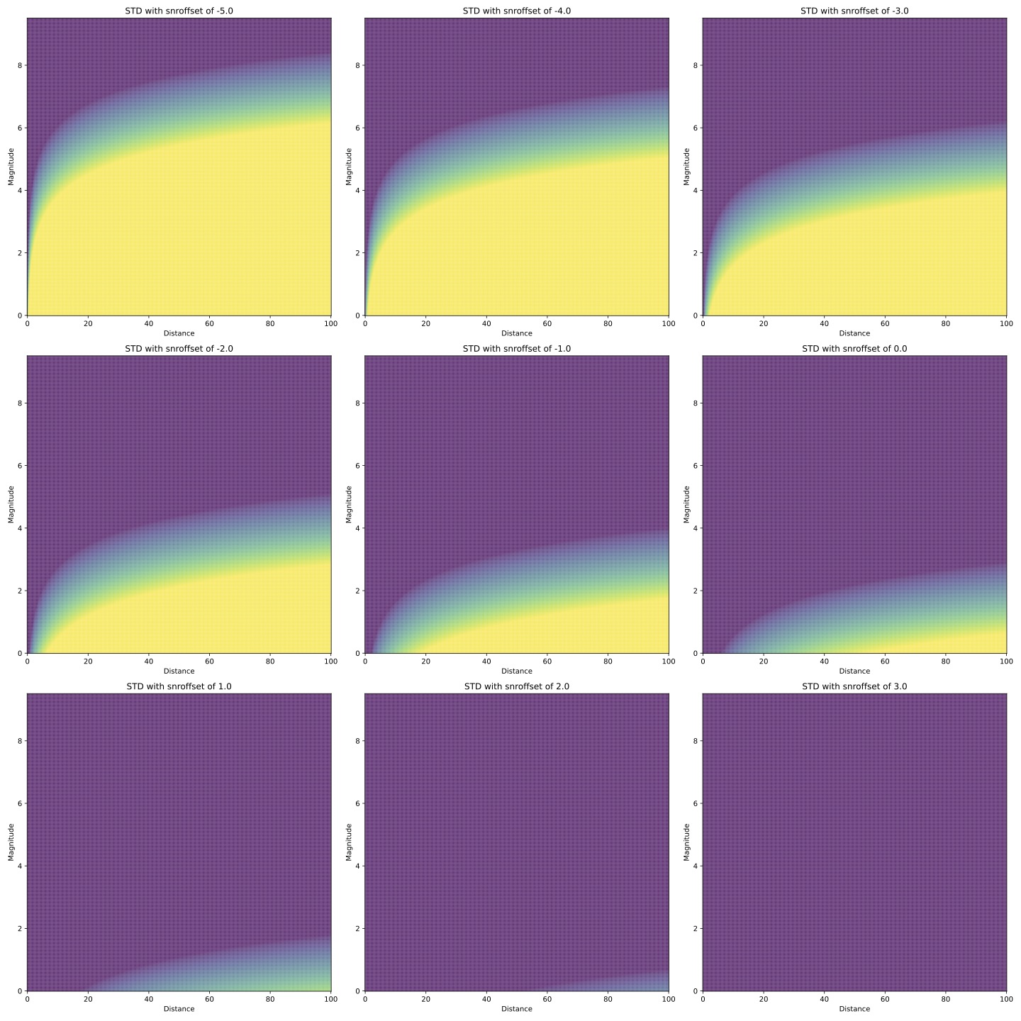
This augmented SNR is then converted to a standard deviation for use in a normal distribution modeling arrival times according to the following equation:

\[\begin{split}\sigma_{meas}(SNR) = \begin{cases} \sigma_0 & \text{SNR} < t_L \\ \gamma\sigma_0 & \text{SNR} > t_U \\ \sigma_0 - \frac{\sigma_0 - \gamma\sigma_0}{\log(t_U) - \log(t_L)}\log(\frac{SNR}{t_L}) & \text{otherwise} \end{cases}\end{split}\]

where \(\gamma\), \(t_U\) and \(t_L\), and \(\sigma_0\) may all be tuned as hyperparameters. The values for these hyperparameters are currently set as:

\[\begin{split}\begin{aligned} \gamma &= .01\\ \sigma_0 &= 10.0\\ t_L &= 5\\ t_U &= 50. \end{aligned}\end{split}\]

By tuning the sensor fidelity, which can be specified in the sensor parameters in either the eig_calc.py input file or the network_opt.py input file, the user can control the measurement error used to model arrival times.

This table provides a notional description of how the measurement error changes as the SNR offset is changed. The first column shows the offset value, and the second two columns show the average measurement error across all events sampled from the given prior for sensors with the given offset. It appears that between values of 1.73 and -0.64, the average measurement error is more sensitive to changes in SNR.

SNR offset	\(\sigma_{meas}\), uniform prior	\(\sigma_{meas}\), nonuniform prior
3.5	0.1	0.1
2.91	0.1	0.1
2.32	0.13	0.15
1.73	0.23	0.38
1.14	0.41	0.75
0.55	0.62	1.19
-0.05	0.81	1.5
-0.64	0.92	1.83
-1.23	0.97	1.94
-1.82	0.99	1.98
-2.41	1.0	1.99
-3.0	1.0	2.0

The figure below shows how the chosen snroffset value of a sensor translates to a measurement error when using a uniform prior.