Performing bounded optimization#
Bounded Optimization#
Both the network analysis code and network optimization code require a domain over which to analyze/optimize. In the latitude/longitude dimensions, this domain can be made up of an arbitrary number of polygonal shapes. This means that the placement of sensors can be constrained according to the needs of the user. Additionally, this means that the seismic events used to analyze networks may also be sampled from an arbitrary latitude/longitude domain. These two domains do not need to be the same, allowing sensors to be placed in a different area than events of interest. Seismic events must also be provided with a range for depth and a range for magnitude from which they can be sampled.
Currently, only a range for depth and magnitude (as opposed to an arbitrary number of polygonal shapes) is supported. These domains should be specified in a boundary constraint file.
Defining the boundary constraint file#
Boundary constraints should be provided in a JSON file. If the sensors and events are to be sampled from the exact same domain, these files may be the same; otherwise, two files must be created.
A constraint file should in the JSON format, which is a lightweight way of storing dictionaries (for more information see the JSON documentation). There are two ways to specify a latitude/longitude constraint:
A set of coordinates. Each coordinate should be of the form (lon, lat) and should be the coordinate of a corner of a polygon defining the bounded domain. Many such sets of coordinates may be provided in order to specify a disconnected domain that consists of several polygonal shapes.
In the case that the optimization domain is a single rectangular region, a latitude range and longitude range may be provided.
These two methods are mutually exclusive. If a latitude/longitude range is provided, a set of coordinates may not be provided, and vice versa. When defining a domain for sampling events, a depth range and magnitude range must also be provided. These specifications are provided in a dictionary format, with each key corresponding to either a range or a set of coordinates. The appropriate keys are specified below:
Dictionary Key |
Description |
|---|---|
|
Range, in list format, from which depth may be sampled for seismic events |
|
Range, in list format, from which magnitude may be sampled for seismic events. This range must be a subset of the range |
|
Range, in list format, from which latitude may be sampled for either seismic events or sensor locations. If this key is included, the |
|
Range, in list format, from which longitude may be sampled for either seismic events or sensor locations. If this key is included, the |
|
Set of coordinates in (longitude, latitude) form where each coordinate defines a corner of a polygon. As many keys specifying sets of coordinates as desired may be included. If any |
|
A second set of coordinates in (longitude, latitude) form where each coordinate defines a corner of a polygon. |
… |
… |
|
The \(N^{th}\) set of coordinates in (longitude, latitude) form where each coordinate defines a corner of a polygon. |
The format for the boundary file when using lat and lon range is:
{"depth_range": [depth_1, depth_2],
         "mag_range": [mag_1, mag_2],
         "lat_range": [lat_1, lat_2],
         "lon_range": [lon_1, lon_2]
        }
while the format for the boundary file when using arrays of coordinates is:
{"depth_range": [depth_1, depth_2],
         "mag_range": [mag_1, mag_2],
         "coordinates_1": [[lon_11, lat_11],
                           [lon_12, lat_12],
                           ...
                           [lon_1n, lat_1n]],
         "coordinates_2": [[lon_21, lat_21],
                           [lon_22, lat_22],
                           ...
                           [lon_2m, lat2m]],
        .
        .
        .
        "coordinates_N": [[lon_N1, lat_N1],
                          [lon_N2, lat_N2],
                          ...
                          [lon_NM, lat_NM]]
        }
Examples#
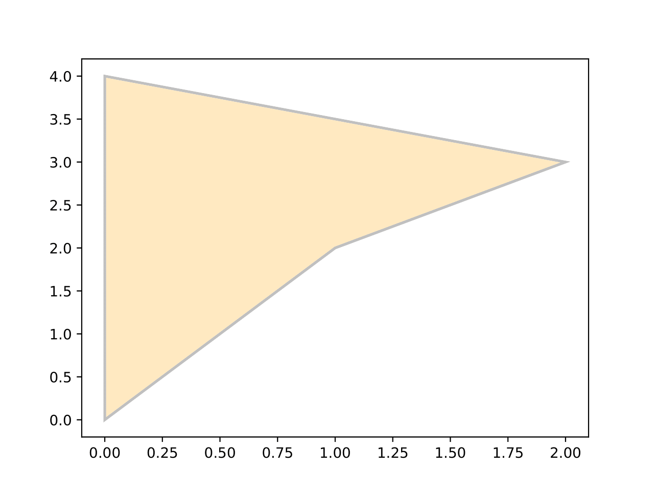
This boundary file:
{"coordinates_1": [[0,1],
                    [0,4],
                    [2,3],
                    [1,2],
                    [0,0],
                    [0,1]]
}
will create a boundary that looks like this:
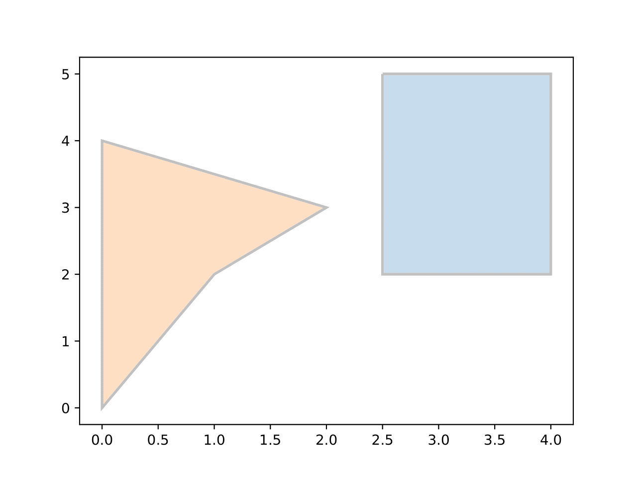
This boundary file:
{"coordinates_1": [[0,1],
                   [0,4],
                   [2,3],
                   [1,2],
                   [0,0],
                   [0,1]],
 "coordinates_2": [[2.5,5],
                   [4,5],
                   [4,2],
                   [2.5,2],
                   [2.5,5]]
}
will create a boundary that looks like this:
Optimizing a network with boundary constraints#
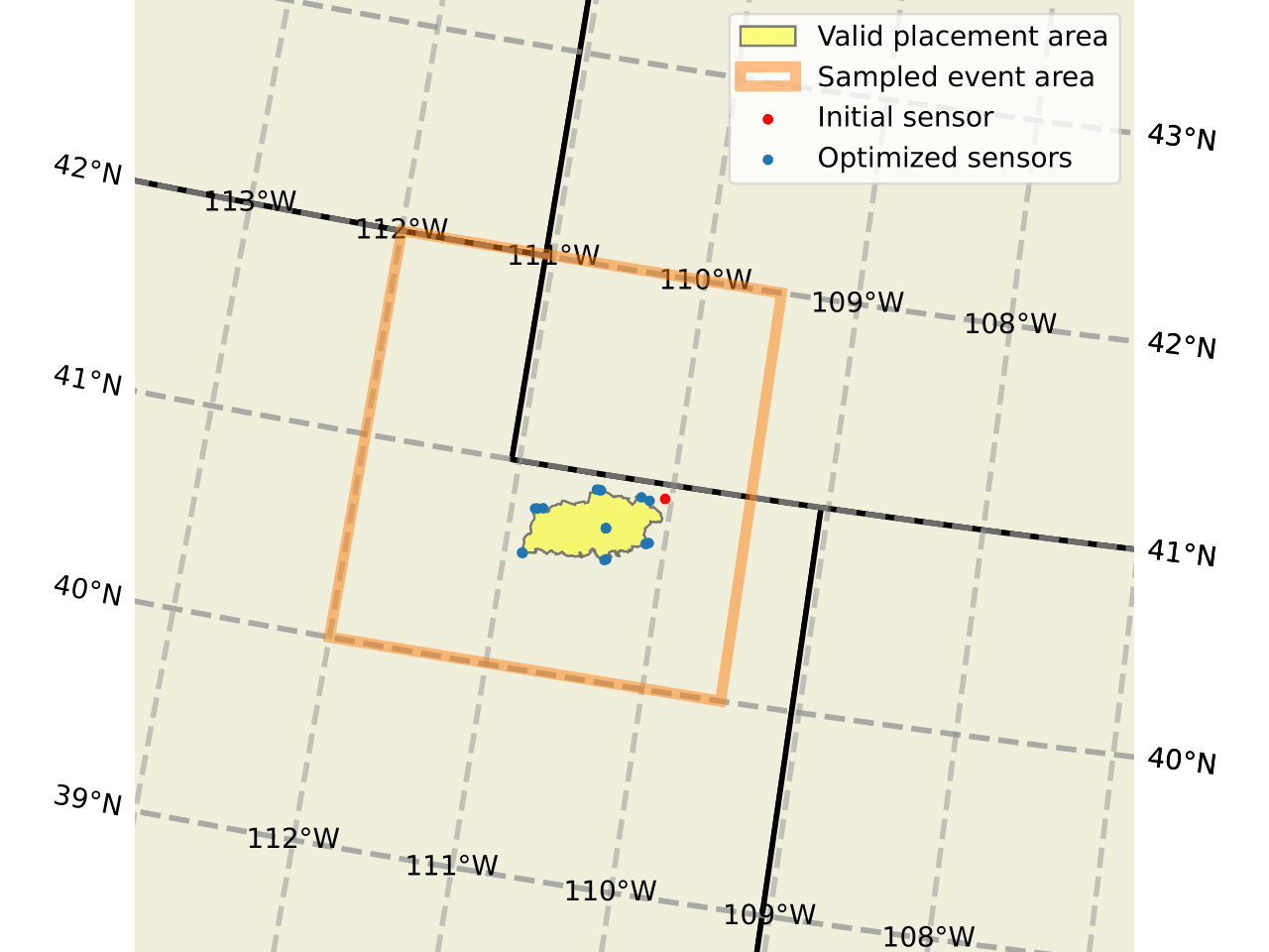
Suppose we’re interested in detecting events inside the area shown by the orange bow below, but it is only possible to place sensors inside the yellow area.
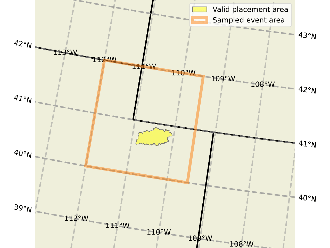
This constraint on sensor placement could be due to state lines, natural features like rivers, man-made features like roads, or other boundaries like state and national forest boundaries.
To accomplish this optimization, we create a boundary file containing the coordinates that define the corners ofthe yellow polygon shown above.
We save the file as example_boundary.json.
Next, we define the input file to the network_opt.py script:
1
20
example_boundary.json
2,2,0
0
1024
4096
2
square_event_coordinates.json
mpiexec --bind-to core --npernode 16 --n 512
unif_prior.py
10
37.,-116.,2.,2.,0.
Here, observe several things about the input file:
Line 3 specifies the filename (and path, if in a different directory) of the shapefile used to define the boundary for the sensors. At this time, a boundary file must always be provided (meaning that if we wanted to simply optimize the sensors over a square domain, we would need to provide a file specifying that).
Line 4 specifies that we wish to use sensors with an SNR offset of 2, an output vector length of 4, and of type
0—meaning sensors that detect seismic waves.Line 10 uses nodes with 36 cores per node and specifies 256 total cores. If the system being used had a different architecture, this line would need to be modified to match the system.
Lines 9 specifies the file defining the boundary from which events may be sampled.
Line 11 specifies the file that contains the proper functions for sampling events (see Writing a sampling file).
For more details on the input file, see Writing an input file.
Now that we have an input file defined, we can run network_opt.py on
Sandia’s HPC clusters as described in Getting started: Network optimization.
We will run interactively: first we’ll request the nodes to use for our job. Running on a system with 16 cores per node, we need to request at least 32 nodes in order to ensure our allocation matches the instructions on line 13 of our input file.
salloc -N 32 -t 8:00:00
Then, we run network_opt.py with Python (for details on the
script arguments see Getting started: Network optimization):
python3 network_opt.py opt_inputs.dat sensor_output.npz output_dir 1
The script will output optimization results after each new sensor is
placed, and will save a .npz file (in this example we called it
sensor_output.npz) containing the final optimized network. These will
be saved in the specified directory (called output_dir in our
example). The network created by our script under our boundary
constraints looks like this: