Getting Started: Network Analysis#
The network analysis code estimates the Expected Information Gain (EIG) of a given seismic monitoring networks for a given prior distribution of potential events. The code samples these candidate events and then generates synthetic datasets that could plausibly be seen by the sensors. For each of the datasets, the code constructs the posterior distribution and computes the information gain (IG) according to the KL-divergence. This information gain is averaged overall synthetic datasets to compute the EIG. The code can also return a list of the IG for different hypothetical events which can be used to generate a map of sensitivities of the network to different event locations, depths, and magnitudes.
The network analysis code is contained in the python script eig_calc.py. This script takes three arguments: a configuration file, an output file location, and a verbosity control. An example configuration file, which we call inputs.dat, might look like this:
128
256
2
ta_array_domain.json
uniform_prior.py
40.0, -111.5,0.1,2,0
41.0, -111.9,0.1,2,0
42.0, -109.0,0.1,2,0
The first line specifies how many events will be used to generate the synthetic data that will be used to compute \(KL\left[p(\theta | D) || p(\theta)\right].\) The second line specifies how many events will be used to discretize the event domain when computing \(KL[p(\theta | D) p(\theta)].\) Line 3 specifies how many realizations of data to generate for each event. Line 4 is the path to the file containing the bounds on the events to be generated, and Line 5 is the path to the file containing the functions for sampling events. For more information on input files, For more information on input files, see Writing input files.
Running the code#
The code can be run interactively, either locally or on an HPC system, or it can be run through a HPC scheduler. This tutorial assumes the HPC system uses Slurm.
The code for analyzing hte network is contained in the Python file eig_calc.py, which is executed with the with the following arguments:
Input file: path to the input file (see Writing input files for more details)
Output Numpy file: Path to the location and filename where the outputs will be saved. File must be in
.npzformat.Verbosity: One of 3 verbosity levels may be specified:
0,1, or2:0has no output other than the final EIG estimate, EIG Standard Deviation, and Statistic of EIG effective sample size.1is the most verbose with printed statements throughout the code describing what is going on and all the different calculated quantities are stored in the output file.2is a more limited version of 1 with less IO and quantities stored in the output file. See Code outputs for a list of which quantities are stored in the output file for each verbosity level.
Running locally#
To run the code on a local machine, execute it with mpi like so:
mpiexec -n 4 python3 eig_calc.py inputs.dat outputs.npz 1
The flag -n specifies how many cores mpiexec should use to execute eig_calc.py.
Running using HPC interactively#
To submit an interactive job, use the salloc command. The command
salloc requests a slurm allocation, and has several flags that are
used to specify the details of the allocation. This varies by system,
but typically the number of nodes and the allocation time are required:
-nodes: The number of nodes to request.--time: The time the nodes will be allocated to your account
An example job allocation request looks like this:
salloc --nodes=2 --time=2:00:00
This command is requesting 2
nodes for a length of 2 hours. For more details on salloc, see the
Slurm documentation: https://slurm.schedmd.com/documentation.html.
Once you have an allocation, you can now submit the job. This is done
with the mpiexec command which requires the following arguments:
--bind-to-core: Binds each process to a physical core--npernode: Specifies the number of cores per node--n: Specifies the total number of available coresExecutable to be run with mpi along with all the arguments to the executable.
In our case, the executable is eig_calc.py with its subsequent arguments as defined above.
For example, to run a job on a machine that has 16 cores per node, we could use the following:
mpiexec --bind-to core --npernode 16 --n 32 python3 eig_calc.py inputs.dat outputs.npz 1
which submits a job using 2 nodes (16 cores per node times 2 nodes gives
32 total cores), reads the input data from inputs.dat, saves the
output data to outputs.npz, and uses verbose setting 1.
Running on HPC with script#
A bash script can be written that will submit a job to the HPC job queue. This does not require the user to specifically allocate nodes to use for the job; nodes will be allocated and the job will begin automatically once the number of nodes specified in the bash script are available. An example script might look like
#!/bin/bash
## Do not put any commands or blank lines before the #SBATCH lines
#SBATCH --nodes=16                   # Number of nodes - all cores
                                     #per node are allocated to the job
#SBATCH --time=04:00:00              # Wall clock time (HH:MM:SS) -
                                     # once the job exceeds this time, the job will be terminated (default is 5 minutes)
#SBATCH --job-name=seis_eig          # Name of job
#SBATCH --export=ALL                 # export environment variables from the submission env
                                     # (modules, bashrc etc)

nodes=$SLURM_JOB_NUM_NODES           # Number of nodes - the number of
                                     # nodes you have requested (for a
                                     # list of SLURM environment
                                     # variables see "man sbatch")
cores=16                             # Number MPI processes to run
                                     # on each node (a.k.a. PPN)


mpiexec --bind-to core --npernode $cores --n $(($cores*$nodes)) python3 -u eig_calc.py inputs.dat outputs.npz 0
This script can then be submitted
using the sbatch command:
sbatch eig_batch_submission_script.bash
For a comprehensive list of available options, see the Slurm documentation (https://slurm.schedmd.com/documentation.html), and in particular the Slurm command/option summary, found here.
Code outputs#
At the end of running eig_calc.py, the code will print to screen the
following results:
Expected information gain (EIG) of the sensor network
Standard deviation (STD) of the expected information gain
Minimum effective sample size (ESS) for all realizations of synthetic data of the weighted samples that make up the posterior distribution estimate
In some sense, the STD and ESS numbers relate to the variance and bias
of the EIG estimator. Additionally, an output Numpy file (e.g.
outputs.npz) is created. The variables stored in this file depend on
the verbose flag. The table below provides a full description of the output.
Variable Name |
Description |
Verbose Levels |
|---|---|---|
|
Estimated expected information gain (EIG) over all experiments |
0, 1, 2 |
|
Standard deviation of EIG over all experiments |
0, 1, 2 |
|
Information gain assessed for each experiment |
1, 2 |
|
Effective sample size (ESS) of weighted posterior samples for each experiment |
1, 2 |
|
Minimum ESS over all experiments |
1,2 |
|
Parameters (latitude, longitude, depth, magnitude) of synthetic events |
1, 2 |
|
Parameters (latitude, longitude, depth, magnitude) that define the posterior event space |
1, 2 |
|
Sensor network configuration as defined in the input file |
1, 2 |
|
Latitude range of events as defined in the input file |
1, 2 |
|
Longitude range of events as defined in the input file |
1, 2 |
|
Depth range of events as defined in the input file |
1, 2 |
|
Magnitude range of events as defined in the input file |
1, 2 |
|
Log-likelihood of candidate event for every synthetic experiment |
1 |
|
Data used in each synthetic experiment |
1 |
Examples#
The prior distribution encodes the experimenter’s a priori belief about the quantities of interest \(\theta\) before observing any data. In this case, the quantities of interest describe a seismic source: $\(\theta = [\verb|latitude, longitude, depth, magnitude|]\)$.
We assume that each variable is independent, so the prior is
In both cases, we analyze a simple network that looks like this:
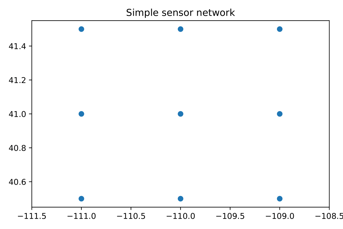
Fig. 1 Example sensor domain#
In each example, we will use 4096 events in a space that’s discretized by 16,384 events. We’ll create 32 realizations of data for each sensor, and we’ll work in a lat/lon domain as shown in the example sensor domain figure, a depth domain of [0,40] and a magnitude domain of [.5,9.5].
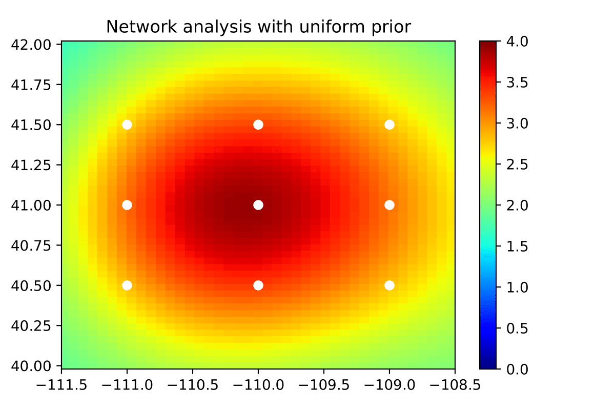
Analysis with uniform prior#
In this example, we assume a uniform distribution on latitude, longitude, and depth, and assume magnitude follows an exponential distribution:
The functions that perform the sampling operations for \(\theta\) can be found in the file uniform_prior.py.
For more information on how to write a sampling file, see #TODO.
These sensors are all of type 0, meaning they produce data based on
seismic waves, and they have a uniform SNR offset value of 0. We first
need to write an input file according to the guidelines in Section
[subsec:input_file]{reference-type=”ref”
reference=”subsec:input_file”}. This input file can be the exact same no
matter what prior we use, with the only change being in Line 8 where the
sampling file is specified. Once this line has been specified correctly,
all other steps will be the same.
Input file#
The input file we will use looks like this:
4096
16384
32
uniform_prior.py
40.5,-109,0,2.,0.
40.5,-110,0,2.,0.
40.5,-111,0,2.,0.
41,-109,0,2.,0.
41,-110,0,2.,0.
41,-111,0,2.,0.
41.5,-109,0,2.,0.
41.5,-110,0,2.,0.
41.5,-111,0,2.,0.
Notice that we’ve specified our choice of prior in line 4, where we’ve provided the path to the file containing our sampling functions, and lines 5 and onward specify the sensor locations. For more information on how the input file is constructed, see Writing input files.
Executing the example#
Once we’ve written an input file, the code can be run using any of the methods described in Running the code. For example, to run interactively on a system with 16 cores per node, we could request 16 nodes:
salloc --nodes=32 --time=8:00:00
and then run the eig_calc.py script:
mpiexec --bind-to core --npernode 16 -n 512 python3 eig_calc.py uniform_inputs.dat uniform_outputs.npz 1
Visualizing outputs#
This code will produce outputs according to Section 3.3, and those outputs can be visualized in a variety of ways.
For example, we could visualize the Expected Information Gain that the network would provide for all events in the domain. When using verbosity level 1, the analysis code saves the KL divergence for all 4096 * 32 sampled datasets. We can load these data and then average across data realizations to compute the Information Gain for each sampled event. We can also load the latitude and longitude domain inside which the events were sampled and the sensor network that we analyzed:
import numpy as np
# Load outputs
output_data = np.load('uniform_outputs.npz')

# Get events
thetas = output_data['theta_data']

# Get ig values for each event
kls = output_data['ig'].reshape((4096, 32))
igs = kls.mean(axis=1)

# Get theta domain
lat_range = output_data['lat_range']
lon_range = output_data['lon_range']

# Get sensors, only store latitude and longitude
sensors = output_data['sensors'][:,:2]
Then, we can fit a surrogate to the Information Gain values and predict the values at all the non-sampled points
Show code cell source
# Visualization helper functions
def select_training_samples(samples,
                            targets,
                            depth_slice=0.5,
                            mag_slice=0.5,
                            depth_tol=5,
                            mag_tol=.75,
                            method='tol',
                            verbose=0
                           ):
    if method=='tol':
        depth_low = depth_slice - depth_tol
        depth_high = depth_slice + depth_tol

        mag_low = mag_slice - mag_tol
        mag_high = mag_slice + mag_tol

        # Mask that selects samples whose magnitude and depth are in the desired range
        mask = [((samples[:,2]<=depth_high) & (samples[:,2]>=depth_low)) &
                ((samples[:,3]<=mag_high) & (samples[:,3]>=mag_low))]

        training_inputs = samples[tuple(mask)]
        training_targets = targets[tuple(mask)]
        if verbose==1:
            print(f'Selected {training_inputs.shape[0]} samples to train with')

    elif method=='random':
        idx = random.sample(range(0,len(samples)), 1000)
        training_inputs = samples[idx]
        training_targets = targets[idx]

    return training_inputs, training_targets

def plot_ig_surface(model,
                 lat_range,
                 lon_range,
                 depth_slice=0.5,
                 mag_slice=0.5,
                 gridsize=50,
                 plot_title="EIG plot"
                ):
    # Create domain points to predict on
    x = np.linspace(lat_range[0], lat_range[1], gridsize)
    y = np.linspace(long_range[0], long_range[1], gridsize)
    xv, yv = np.meshgrid(x, y)
    xy = np.column_stack((xv.ravel(), yv.ravel())).T

    # Give each lat/lon domain point a depth and magnitude
    domain = np.zeros((len(xy), 4))
    domain[:, :2] = xy
    domain[:, 2] = depth_slice
    domain[:, 3] = mag_slice

    # Predict IG value at each domain point
    preds = model.predict(domain)

    # Plot predictions with longitude for x and latitude for y
    # Note that this is opposite of how the code processes them
    im = plt.pcolormesh(yv,
                        xv,
                        preds.reshape((gridsize, gridsize)),
                        shading="auto",
                        cmap="jet"
                       )
    im.set_clim(preds.min(),preds.max()) # Standardize colorbar limits

    # Plot sensor network on map
    plt.scatter(net[:, 1],net[:, 0],c="white", label="sensors")

    # Plot decorations
    plt.title(plot_title)
    ax.set_xlabel("Longitude")
    ax.set_ylabel("Latitude")

    plt.show()
from sklearn.gaussian_process import GaussianProcessRegressor as GPR
from skopt.learning.gaussian_process.kernels import RBF, WhiteKernel

# Downsample training data since a GP will take a long time to train with 4096 points
training_samples, training_targets = select_training_samples(thetas, igs)

# Create and fit the model
kernel = (1.0 *
          RBF(length_scale=[1.0, 1.0,1.0,1.0], length_scale_bounds=(0.2, 1)) +
          WhiteKernel(noise_level=0.1, noise_level_bounds=(1e-2, 5e-1))
         )
model = GPR(kernel=kernel,alpha=0.0, normalize_y=True)
model.fit(training_samples, training_targets)
Then we can make predictions on the whole domain and visualize the predictions:
plot_ig_surface(model,
                lat_range,
                lon_range,
                plot_title="Network analysis with uniform prior"
               )
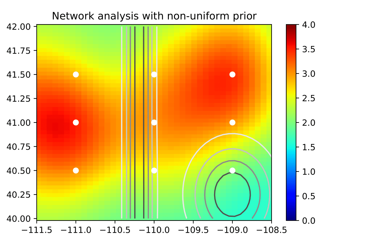
Analysis with nonuniform prior#
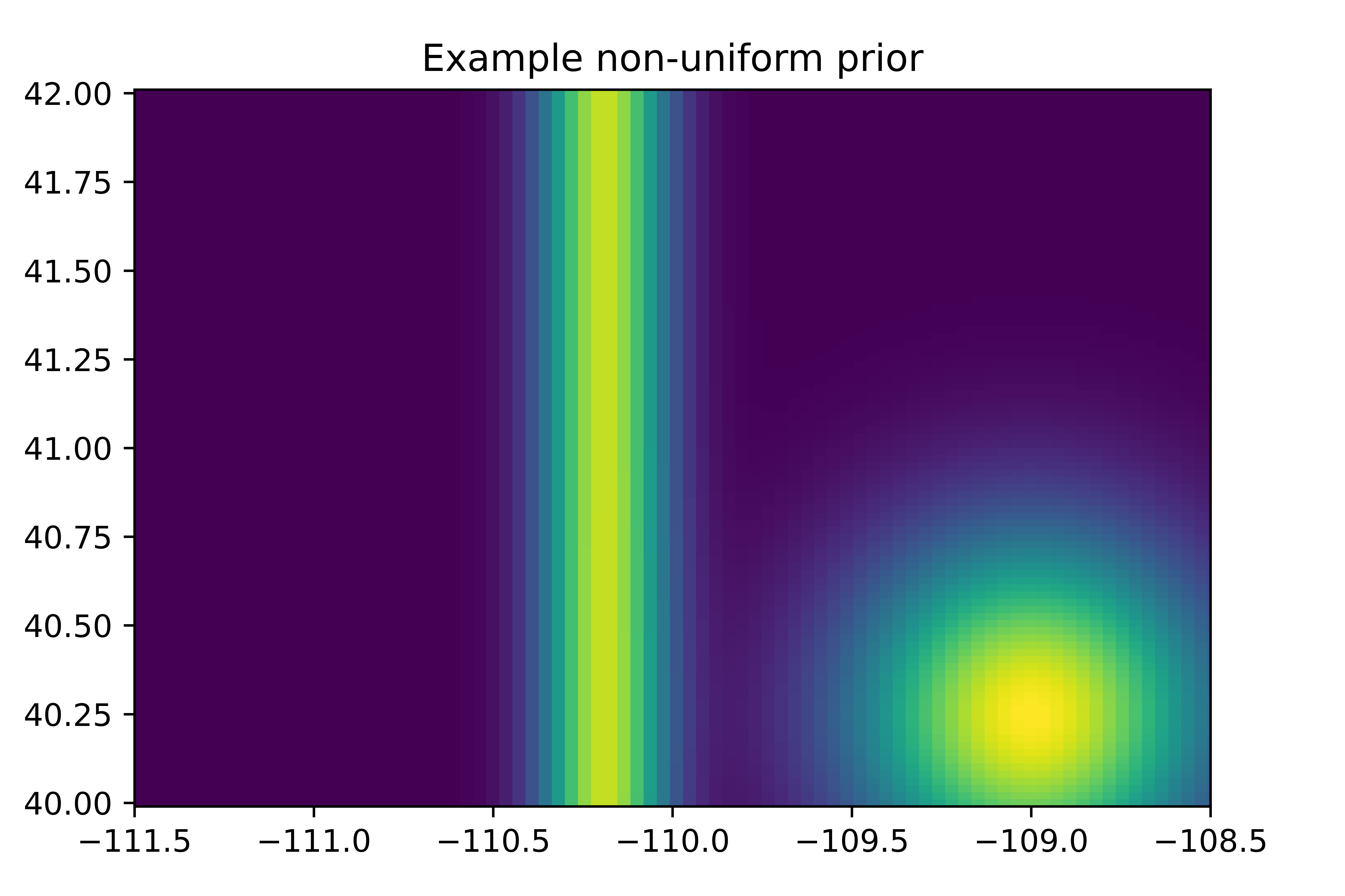
Instead of a uniform prior on seismic event locations, in this example we will assume depth is uniformly distributed and magnitude follows the same exponential distribution as in the previous example, but in this example we will assume location (latitude and longitude) follows a Gaussian mixture distribution as shown in this figure:
The functions that perform the sampling operations for \(\theta\) can be found in the file nonuniform_prior.py.
For more information on how to write a sampling file, see #TODO.
Inputs#
The input file we use for this example will be almost identical to the uniform prior example, with the only change being the line providing the path to the sampling file:
4096
16384
32
nonuniform_prior.py
40.5,-109,0,2.,0.
40.5,-110,0,2.,0.
40.5,-111,0,2.,0.
41,-109,0,2.,0.
41,-110,0,2.,0.
41,-111,0,2.,0.
41.5,-109,0,2.,0.
41.5,-110,0,2.,0.
41.5,-111,0,2.,0.
Executing the example#
We will execute the network analysis the same way as in the uniform example, but we re-emphasize that any of the methods described in Running the code will work. On a system with 16 cores per node, we request 16 nodes:
salloc --nodes=32 --time=8:00:00
and then run the eig_calc.py script:
mpiexec --bind-to core --npernode 16 -n 512 python3 eig_calc.py nonuniform_inputs.dat nonuniform_outputs.npz 1
Visualizing the results#
We will visualize the results similarly to the previous example by creating a surface predicting the Expected Information Gain at each point in the lat/lon domain. We load the outputs of the analysis with the nonuniform prior:
import numpy as np
# Load outputs
output_data = np.load('nonuniform_outputs.npz')

# Get events
thetas = output_data['theta_data']

# Get ig values for each event
kls = output_data['ig'].reshape((4096, 32))
igs = kls.mean(axis=1)

# Get theta domain
lat_range = output_data['lat_range']
lon_range = output_data['lon_range']

# Get sensors, only store latitude and longitude
sensors = output_data['sensors'][:,:2]
Next, we fit a surrogate to the Information Gain values and predict the values at all the non-sampled points
# Downsample training data since a GP will take a long time to train with 4096 points
training_samples, training_targets = select_training_samples(thetas, igs)

# Create and fit the model
kernel = (1.0 *
          RBF(length_scale=[1.0, 1.0,1.0,1.0], length_scale_bounds=(0.2, 1)) +
          WhiteKernel(noise_level=0.1, noise_level_bounds=(1e-2, 5e-1))
         )
model = GPR(kernel=kernel,alpha=0.0, normalize_y=True)
model.fit(training_samples, training_targets)
Then we can make predictions on the whole domain and visualize the predictions:
plot_ig_surface(model,
                lat_range,
                lon_range,
                plot_title="Network analysis with nonuniform prior"
               )